JN6: Practice Activity 5#
In this interactive activity, you will learn about two methods that you can use on a ReferenceFrame to define its angular velocity (and, therefore, also its angular acceleration).
Case 1: Given just orientation angle between two frames#
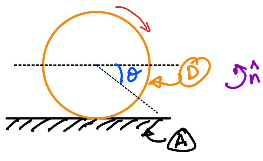
The figure below is that of the rolling disk, which was covered in the lecture (see your notes file titled “6 rigid body kinematics: angular velocities and accelerations.pdf”)

Fig. 9 Motion of a rolling disk \(D\) relative to ground \(A\).#
You can see that the information given here is:
the angle \(\theta\) between frames \(A\) and \(D\); and
direction of rotation of the disk.
You can use this information to define the orientation of \(D\) and \(A\), as follows.
First we use dynamicsymbols to create the variable theta to represent the angle shown in the picture:
from sympy.physics.mechanics import dynamicsymbols, ReferenceFrame
theta = dynamicsymbols('theta')
---------------------------------------------------------------------------
ModuleNotFoundError                       Traceback (most recent call last)
Cell In[1], line 1
----> 1 from sympy.physics.mechanics import dynamicsymbols, ReferenceFrame
      2 theta = dynamicsymbols('theta')

ModuleNotFoundError: No module named 'sympy'
Then, we represent \(A\) and \(D\) by creating two ReferenceFrame using the variables A and D, as shown below:
A = ReferenceFrame('A')
D = ReferenceFrame('D')
Then, we can provide information regarding the rotation of D relative to A by using D.orient, as below; this is a method that we apply to the variable D with the negative of the angle (can you remember why?):
D.orient(A, 'Axis', (-theta, A.z))
The orient method takes the following sequence of information in the parantheses:
Frame of rotation, in this case,
Athe type of rotation, in this case it is the
Axis(however, we will learn to provide it DCMs in the next notebook); anda pair of values in round brackets, containing the angle and the specific axis of rotation. __ You will get an error (or incorrect result) if you do not provide the information in the order listed above__.
You can now see that sympy has the power to automatically compute \(^A\omega^D\). In other words, this is the angular velocity of D in A; you can see that this has been done by using the .ang_vel_in method:
D.ang_vel_in(A)
In fact, sympy also has the power to automatically compute the angular acceleration of D in A, as shown below:
D.ang_acc_in(A)
sympy can also generate \(^D {\bf C} ^A\) the direction cosine matrix of \(A\) relative to \(D\).
D.dcm(A)
As you can imagine, this is incredibly powerful because sympy can automatically compute the rotational kinematics as long as you provide sympy the correct information in the orient method: direction of rotation angle (-theta), type of rotation (Axis), and axis of rotation (A.z).
Case 2: If you are only given angular speed and direction of rotation then you should use the .set_ang_vel#
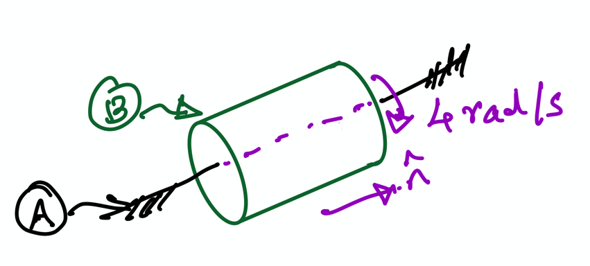
In some cases, you are not given an orientation angle. Instead, you are given the angular speed and the direction of rotation. An example of this is the rotating shaft (shown below and also covered in the lecture):

Fig. 10 Motion of a shaft \(B\) rotating relative to fixed axis \(A\).#
The shaft is rotating at the constant speed \(4\) radian per second. So, from the figure, we can easily infer that the \(^A\omega^B = 4 \hat{\bf n} = 4 \hat{\bf a}_z\). Here, we made the assumption that \(\hat{\bf n} = 4 \hat{\bf a}_z\). Let’s see how we can let provide this information to sympy.
First, we create the \(A\) and \(B\) frames using ReferenceFrame; the frames are assigned the variable names A and B:
A = ReferenceFrame('A')
B = ReferenceFrame('B')
Then, we can can define \(^A\omega^B\) using a new method on B; this method is called set_ang_vel. This is done as shown:
B.set_ang_vel(A, 4*A.z)
The sequence of information in the set_ang_vel is:
The frame relative to which we define the orientation. In this example, it is
A.The vector expression of the angular velocity. In this example, it is
4*A.z.
We can examine that the angular velocity is indeed assigned to B by using the ang_vel_in command (which was described in the above subsection on rolling disk). We can do this in the following way:
B.ang_vel_in(A)
\(^A\alpha^B\), the angular acceleration of B in A, has also been automatically computed:
B.ang_acc_in(A)
This should be zero because the rotation speed is constant i.e., \(4\) rad/s.
Though the information on angular velocity and acceleration is automatically computed, extracting the direction cosine matrix is not possible as the angle is not specified in the problem statement. Thus, if you try to run B.dcm(A), an error message will appear.
B.dcm(A)
---------------------------------------------------------------------------
ValueError                                Traceback (most recent call last)
<ipython-input-12-2cf0bbadf61d> in <module>
----> 1 B.dcm(A)

~/opt/anaconda3/lib/python3.7/site-packages/sympy/physics/vector/frame.py in dcm(self, otherframe)
    426         if otherframe in self._dcm_cache:
    427             return self._dcm_cache[otherframe]
--> 428         flist = self._dict_list(otherframe, 0)
    429         outdcm = eye(3)
    430         for i in range(len(flist) - 1):

~/opt/anaconda3/lib/python3.7/site-packages/sympy/physics/vector/frame.py in _dict_list(self, other, num)
    271             return outlist[0]
    272         raise ValueError('No Connecting Path found between ' + self.name +
--> 273                          ' and ' + other.name)
    274
    275     def _w_diff_dcm(self, otherframe):

ValueError: No Connecting Path found between B and A
So, ultimately, the problem and assoicated figure dictates whether one uses .orient or .set_ang_vel on a ReferenceFrame variable in defining the orientation kinematics.


