Radial Burn#
In radial burn, combustion starts along the symmetry axis and proceeds radially outwards. Thus, at any instant, the unburned portion resembles a hollow pipe and both the axial and transverse radius of gyration of the system are variable as shown in Figure Fig. 11.
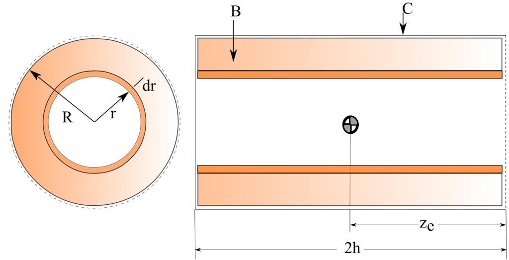
Fig. 11 Radially burning cylinder.#
For the results presented here, the initial radius and length are \(1\) m. The instantaneous moment of inertia scalars for the radially burning cylinder are
and
Their corresponding time derivatives are
The angular speeds evaluate to
Evidently, the spin rate is not constant for a cylinder subject to radial burn. It varies such that it appears to damp out, slowly, for about two-thirds of the burn. Towards the end of the burn, i.e., as \(r\) approaches \(R\), the spin rate grows without bounds. Analytically, this growth in spin rate has been found to begin at the instant \(r/R = 0.707\) [Mao and Eke, 2000]. The transverse angular speed, on the other hand, can either grow, decay, or fluctuate depending on the shape of the cylinder before the start of the burn. The corresponding body and space surfaces for the radially burning cylinder are shown in Figures Fig. 12 and Fig. 13, respectively, for a burn duration of \(90\) s; this duration is chosen purely to study a case where the end mass of the system approaches the mass of a payload.
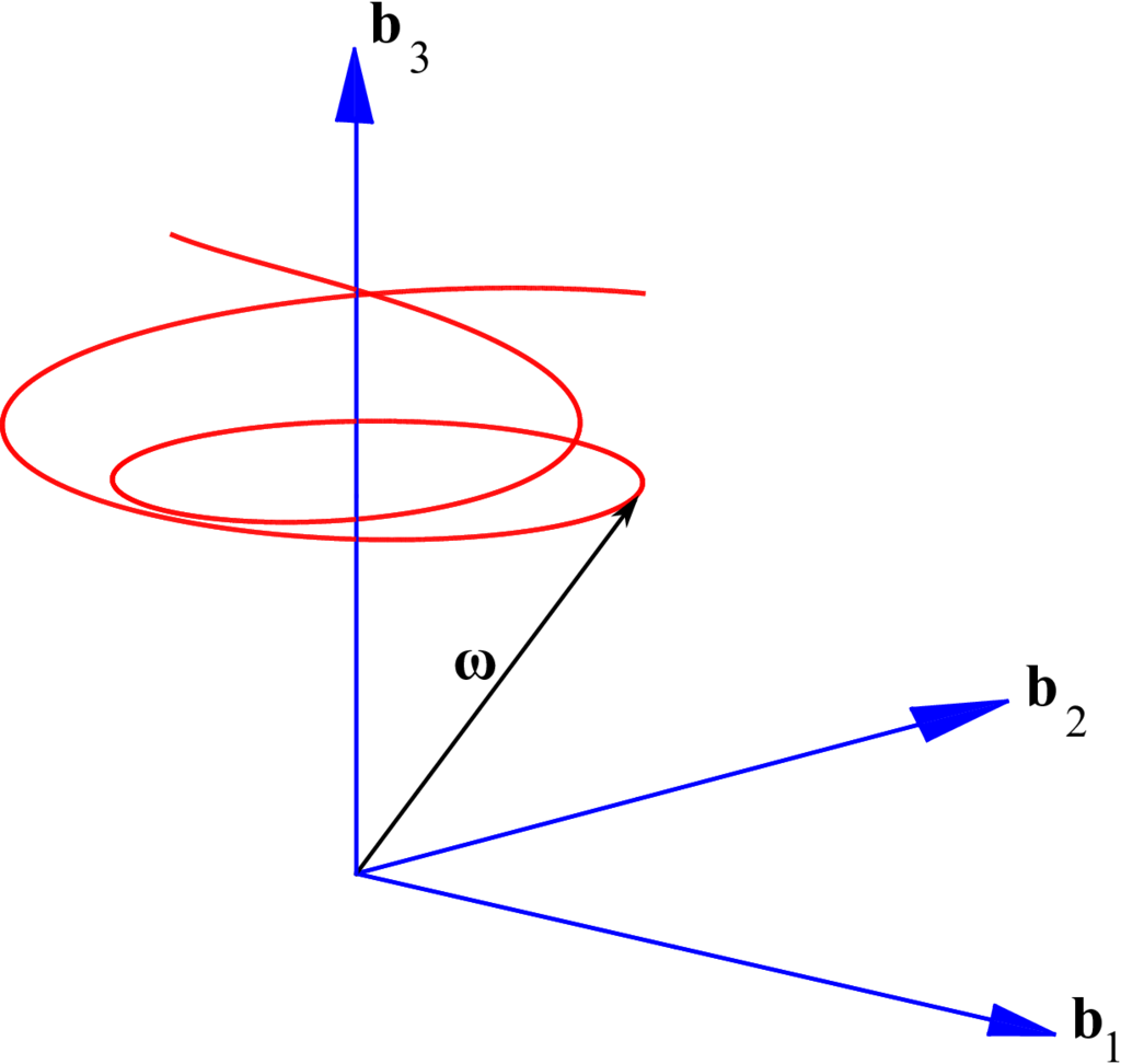
Fig. 12 Radial burn: body surface.#
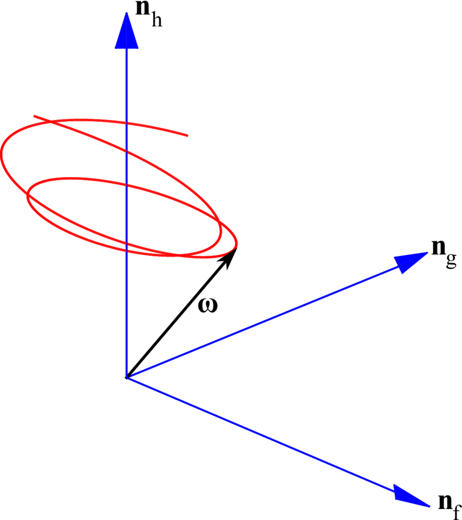
Fig. 13 Radial burn: space surface.#
The case presented here is for \(R/h=2\) and is a nutationally stable configuration; this is in agreement with Mao and Eke’s work [Mao and Eke, 2000] where it was shown that transverse rates are unbounded for oblate radially burning cylinders with a \(R/h \geq \sqrt{8/3}\). The cone angle does in fact monotonically decrease though this is not as evident from Figure Fig. 12 when compared to the uniform and end burns; this is primarily due to the fact that the system’s end mass is approximately 315 kg at the end of this radial burn whereas in the other burns it is nearly zero. One approach to verifying the nutational stability of the system is by plotting the time evolution of \(\theta\). However, the stability can also be verified from the angular speeds. For the extreme case of oblateness represented by a radially burning flat disk (i.e., \(R \gg h\)), Equation eq68 can be reformulated as
by dropping the terms involving \(h\) from the solution to the transverse speed. Extending this rationale to the inertia scalars given by Equations (58) and (59), we also get \(I/J = 1/2\). Then, the nutation angle from Equation (39) can be expressed as
which is clearly bounded. In other words, even the most oblate configuration of a radially burning cylinder results in a constant nutation angle and thus does not show growth in the coning motion. However, unlike the preceding burns, the radial burn would require a nutation damper system to attenuate the cone angle and bring the system into a state of pure spin.
Simulation Results#
import numpy as np
from scipy.integrate import solve_ivp
import matplotlib.pyplot as plt
from matplotlib.animation import FuncAnimation
Intel MKL WARNING: Support of Intel(R) Streaming SIMD Extensions 4.2 (Intel(R) SSE4.2) enabled only processors has been deprecated. Intel oneAPI Math Kernel Library 2025.0 will require Intel(R) Advanced Vector Extensions (Intel(R) AVX) instructions.
Intel MKL WARNING: Support of Intel(R) Streaming SIMD Extensions 4.2 (Intel(R) SSE4.2) enabled only processors has been deprecated. Intel oneAPI Math Kernel Library 2025.0 will require Intel(R) Advanced Vector Extensions (Intel(R) AVX) instructions.
Define the global physical parameters for the variable mass system#
rho_ini = 1020
rho_exhaust = 0.002 * rho_ini
L = 1  # m
h = L / 2  # m
R = L  # m
u = 5  # m/s
m_dot = -rho_exhaust * u * np.pi * R**2
w0 = 0.2  # rad/s
Initial angular rates#
w10 = 0  # rad/s
w20 = w0  # rad/s
w30 = 0.3  # rad/s
Initial mass properties#
mf0 = np.pi * R**2 * L * rho_ini  # kg
I10 = mf0 * (R**2 / 4 + h**2 / 3)  # kg*m^2
I30 = mf0 * R**2 / 2  # kg*m^2
chi0 = 0  # Initial precession angle
Fd0 = 0  # Initial F value
tb = -mf0 / m_dot - 1  # Burn time
Quaternion initial conditions (representing no initial rotation)#
q0 = [1, 0, 0, 0] # (w, x, y, z)
Combine initial conditions#
Y0 = [mf0, I10, I30, w10, w20, w30, chi0, Fd0] + q0
Define the differential equations#
def uniburn(t, w):
    m, I1, I3, w1, w2, w3, chi, F, qw, qx, qy, qz = w
    # Mass varying terms
    md = -rho_exhaust * np.pi * R**2 * u  # mass
    I1d = md * (R**2 / 4 + h**2 / 3)  # transverse moment of inertia
    I3d = md * R**2 / 2  # spin moment of inertia
    # Equations of motion for the axisymmetric cylinder undergoing uniform burn
    w1d = (I1 - I3) * w2 * w3 / I1 - (I1d - md * (h**2 + R**2 / 4)) * w1 / I1
    w2d = -(I1 - I3) * w1 * w3 / I1 - (I1d - md * (h**2 + R**2 / 4)) * w2 / I1
    w3d = -(I3d - md * R**2 / 2) * w3
    chid = (1 - I3 / I1) * w3
    Fd = -(I1d - md * (h**2 + R**2 / 4)) / I1
    # Quaternion derivative
    omega_quat = np.array([0, w1, w2, w3])
    quat = np.array([qw, qx, qy, qz])
    quat_dot = 0.5 * np.array(quat_mult(quat, omega_quat))
    wd = [md, I1d, I3d, w1d, w2d, w3d, chid, Fd, quat_dot[0], quat_dot[1], quat_dot[2], quat_dot[3]]
    return wd
Function to multiply two quaternions#
def quat_mult(q, r):
    w1, x1, y1, z1 = q
    w2, x2, y2, z2 = r
    return [
        w1*w2 - x1*x2 - y1*y2 - z1*z2,
        w1*x2 + x1*w2 + y1*z2 - z1*y2,
        w1*y2 - x1*z2 + y1*w2 + z1*x2,
        w1*z2 + x1*y2 - y1*x2 + z1*w2
    ]
Time span for the simulation#
dt = 0.01
t_eval = np.arange(0, tb, dt)
Solve the ODEs#
sol = solve_ivp(uniburn, [0, tb], Y0, t_eval=t_eval, atol=1e-9, rtol=1e-8)

# Extract results if the integration was successful
if sol.status == 0:
    print("Integration successful.")
    t = sol.t
    m = sol.y[0]
    I1 = sol.y[1]
    I3 = sol.y[2]
    omega1 = sol.y[3]
    omega2 = sol.y[4]
    omega3 = sol.y[5]
    chi = sol.y[6]
    F = sol.y[7]
    qw, qx, qy, qz = sol.y[8], sol.y[9], sol.y[10], sol.y[11]
else:
    print(f"Integration failed with status {sol.status}: {sol.message}")

# Print the final time to check if it reached the end of the burn time
print(f"Final time: {sol.t[-1]}")
Integration successful.
Final time: 99.0
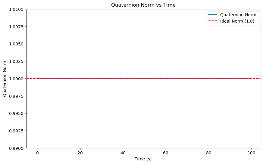
# Plot the quaternion norm over time
quat_norm = np.sqrt(qw**2 + qx**2 + qy**2 + qz**2)
norm_violation_indices = np.where(np.abs(quat_norm - 1) > 1e-6)[0]
if len(norm_violation_indices) > 0:
    print(f"Quaternion constraint violated at time steps: {t[norm_violation_indices]}")
else:
    print("Quaternion constraint satisfied throughout the simulation.")
plt.figure(figsize=(10, 6))
plt.plot(t, quat_norm, label='Quaternion Norm')
plt.axhline(y=1.0, color='r', linestyle='--', label='Ideal Norm (1.0)')
plt.xlabel('Time (s)')
plt.ylabel('Quaternion Norm')
plt.title('Quaternion Norm vs Time')
plt.ylim([0.99, 1.01])  # Adjust y-limits for better visualization
plt.legend()
plt.show()
Quaternion constraint satisfied throughout the simulation.
Function to convert quaternion to Euler angles (Z-X-Z sequence)#
def quat_to_euler_zxz(q):
    """
    Convert a quaternion to Euler angles (Z-X-Z sequence).
    """
    w, x, y, z = q
    # Compute the Euler angles
    psi = np.arctan2(2*(w*z + x*y), 1 - 2*(y**2 + z**2))
    theta = np.arccos(2*(w*y - z*x))
    phi = np.arctan2(2*(w*z + y*x), 1 - 2*(x**2 + y**2))
    return psi, theta, phi
Extract Euler angles from quaternions#
psi, theta, phi = np.zeros(len(qw)), np.zeros(len(qw)), np.zeros(len(qw))
for i in range(len(qw)):
    psi[i], theta[i], phi[i] = quat_to_euler_zxz([qw[i], qx[i], qy[i], qz[i]])
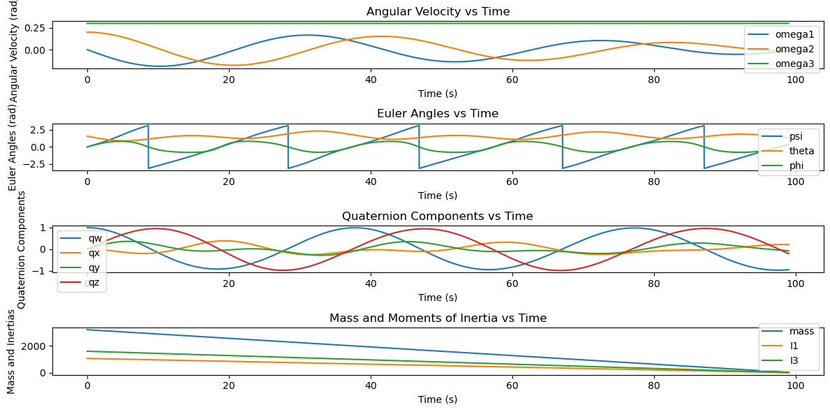
Plot the results#
plt.figure(figsize=(12, 6))

# Plot angular velocities
plt.subplot(4, 1, 1)
plt.plot(sol.t, omega1, label='omega1')
plt.plot(sol.t, omega2, label='omega2')
plt.plot(sol.t, omega3, label='omega3')
plt.xlabel('Time (s)')
plt.ylabel('Angular Velocity (rad/s)')
plt.title('Angular Velocity vs Time')
plt.legend()

# Plot Euler angles
plt.subplot(4, 1, 2)
plt.plot(sol.t, psi, label='psi')
plt.plot(sol.t, theta, label='theta')
plt.plot(sol.t, phi, label='phi')
plt.xlabel('Time (s)')
plt.ylabel('Euler Angles (rad)')
plt.title('Euler Angles vs Time')
plt.legend()

# Plot quaternions
plt.subplot(4, 1, 3)
plt.plot(sol.t, qw, label='qw')
plt.plot(sol.t, qx, label='qx')
plt.plot(sol.t, qy, label='qy')
plt.plot(sol.t, qz, label='qz')
plt.xlabel('Time (s)')
plt.ylabel('Quaternion Components')
plt.title('Quaternion Components vs Time')
plt.legend()

# Plot mass and moments of inertia
plt.subplot(4, 1, 4)
plt.plot(sol.t, m, label='mass')
plt.plot(sol.t, I1, label='I1')
plt.plot(sol.t, I3, label='I3')
plt.xlabel('Time (s)')
plt.ylabel('Mass and Inertias')
plt.title('Mass and Moments of Inertia vs Time')
plt.legend()

plt.tight_layout()
plt.show()
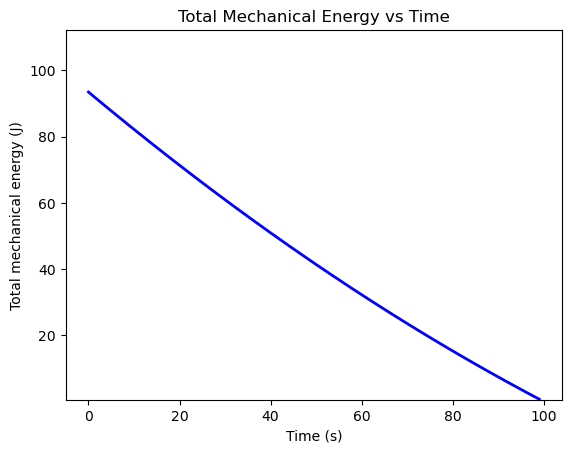
# Plot the T-handle's total mechanical energy over time
E = 0.5 * (I1 * omega1**2 + I1 * omega2**2 + I3 * omega3**2)

plt.figure()
plt.plot(sol.t, E, '-b', linewidth=2)
plt.xlabel('Time (s)')
plt.ylabel('Total mechanical energy (J)')
plt.ylim([min(E) * 0.8, max(E) * 1.2])  # Set fixed y-axis limits
plt.title('Total Mechanical Energy vs Time')
plt.show()

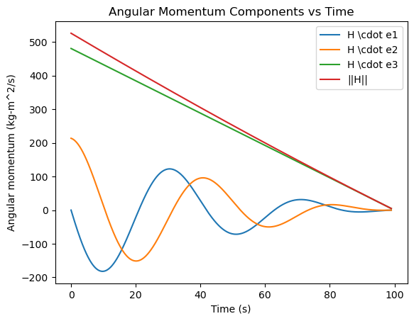
# Plot the components of the angular momentum about the mass center and the total angular momentum over time
H1 = I1 * omega1  # kg-m^2/s
H2 = I1 * omega2  # kg-m^2/s
H3 = I3 * omega3  # kg-m^2/s
H = np.sqrt(H1**2 + H2**2 + H3**2)  # kg-m^2/s

plt.figure()
plt.plot(sol.t, H1, label='H \cdot e1')
plt.plot(sol.t, H2, label='H \cdot e2')
plt.plot(sol.t, H3, label='H \cdot e3')
plt.plot(sol.t, H, label='||H||')
plt.xlabel('Time (s)')
plt.ylabel('Angular momentum (kg-m^2/s)')
plt.title('Angular Momentum Components vs Time')
plt.legend()
plt.show()
# Function to convert quaternion to rotation matrix
def quat_to_rot_matrix(q):
    """
    Convert a quaternion q to a rotation matrix.
    """
    w, x, y, z = q
    return np.array([
        [1 - 2*(y**2 + z**2), 2*(x*y - z*w), 2*(x*z + y*w)],
        [2*(x*y + z*w), 1 - 2*(x**2 + z**2), 2*(y*z - x*w)],
        [2*(x*z - y*w), 2*(y*z + x*w), 1 - 2*(x**2 + y**2)]
    ])

def animate_t_handle_quat(qw, qx, qy, qz, dt):
    # Specify dimensions for the T-handle
    LAG = 0.5  # cm
    LBC = 4  # cm
    LAD = 2  # cm

    # Initialize arrays to store the T-handle's orientation and key points
    e1 = np.zeros((3, len(qw)))
    e2 = np.zeros((3, len(qw)))
    e3 = np.zeros((3, len(qw)))
    xA, yA, zA = np.zeros(len(qw)), np.zeros(len(qw)), np.zeros(len(qw))
    xB, yB, zB = np.zeros(len(qw)), np.zeros(len(qw)), np.zeros(len(qw))
    xC, yC, zC = np.zeros(len(qw)), np.zeros(len(qw)), np.zeros(len(qw))
    xD, yD, zD = np.zeros(len(qw)), np.zeros(len(qw)), np.zeros(len(qw))

    # Calculate the orientation of the T-handle over time
    for k in range(len(qw)):
        q = [qw[k], qx[k], qy[k], qz[k]]
        R = quat_to_rot_matrix(q)
        e1[:, k] = R @ np.array([1, 0, 0])
        e2[:, k] = R @ np.array([0, 1, 0])
        e3[:, k] = R @ np.array([0, 0, 1])
        xA[k] = -LAG * e2[0, k]
        yA[k] = -LAG * e2[1, k]
        zA[k] = -LAG * e2[2, k]
        xB[k] = xA[k] + LBC / 2 * e1[0, k]
        yB[k] = yA[k] + LBC / 2 * e1[1, k]
        zB[k] = zA[k] + LBC / 2 * e1[2, k]
        xC[k] = xA[k] - LBC / 2 * e1[0, k]
        yC[k] = yA[k] - LBC / 2 * e1[1, k]
        zC[k] = zA[k] - LBC / 2 * e1[2, k]
        xD[k] = xA[k] + LAD * e2[0, k]
        yD[k] = yA[k] + LAD * e2[1, k]
        zD[k] = zA[k] + LAD * e2[2, k]

    # Set up the figure window
    fig = plt.figure()
    ax = fig.add_subplot(111, projection='3d')
    ax.set_xlabel('X (cm)')
    ax.set_ylabel('Y (cm)')
    ax.set_zlabel('Z (cm)')
    ax.set_xlim([-LBC, LBC])
    ax.set_ylim([-LBC, LBC])
    ax.set_zlim([-LAD, LAD])
    ax.set_title('T-handle Animation')

    # Draw the T-handle
    AD, = ax.plot([xA[0], xD[0]], [yA[0], yD[0]], [zA[0], zD[0]], 'k-', linewidth=5)
    BC, = ax.plot([xB[0], xC[0]], [yB[0], yC[0]], [zB[0], zC[0]], 'k-', linewidth=5)

    # Animate the T-handle's motion by updating the figure with its current orientation
    def update(k):
        AD.set_data([xA[k], xD[k]], [yA[k], yD[k]])
        AD.set_3d_properties([zA[k], zD[k]])
        BC.set_data([xB[k], xC[k]], [yB[k], yC[k]])
        BC.set_3d_properties([zB[k], zC[k]])
        return AD, BC,

    ani = FuncAnimation(fig, update, frames=len(qw), interval=dt * 1000, blit=True)
    plt.show()

# Example usage
# Assuming `qw`, `qx`, `qy`, `qz` are the quaternion components obtained from the previous solution
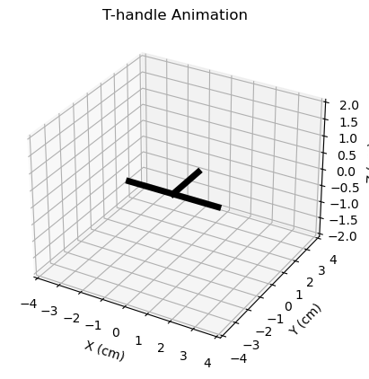
animate_t_handle_quat(qw, qx, qy, qz, dt)
