Two-Body Dynamics

Prepared by: Emmanuel Airiofolo, Joost Hubbard, Ceyda Alan and Angadh Nanjangud

In this lecture we cover the following topics:

1. Two-Body Dynamics

2. Two-Body Relative Dynamics

3. Specific Angular Momentum

4. Kepler’s Second Law

5. Two-body Dynamics in Polar Coordinates

6. Conservation of Specific Orbital Energy: E

7. Admissible Orbital Radius

Two-Body Dynamics

Fig. 1 allows us to modely the two-body dynamics of two particles \(m_1\) and \(m_2\). Their position vectors from \(O\) are given by \({\bf{r}}_1\) and \({\bf{r}}_2\), respectively. Note that \(O\) is the origin of an inertial reference frame. \(G\) is the center of mass of the two-body system, which is located by \(\bf{r}_G\). The relative position vector from \(m_1\) to \(m_2\) is given by \({\bf{r}}\). The unit vectors \(\hat{\bf{i}}\), \(\hat{\bf{j}}\), and \(\hat{\bf{k}}\) form a right-handed orthonormal system for this inertial frame.

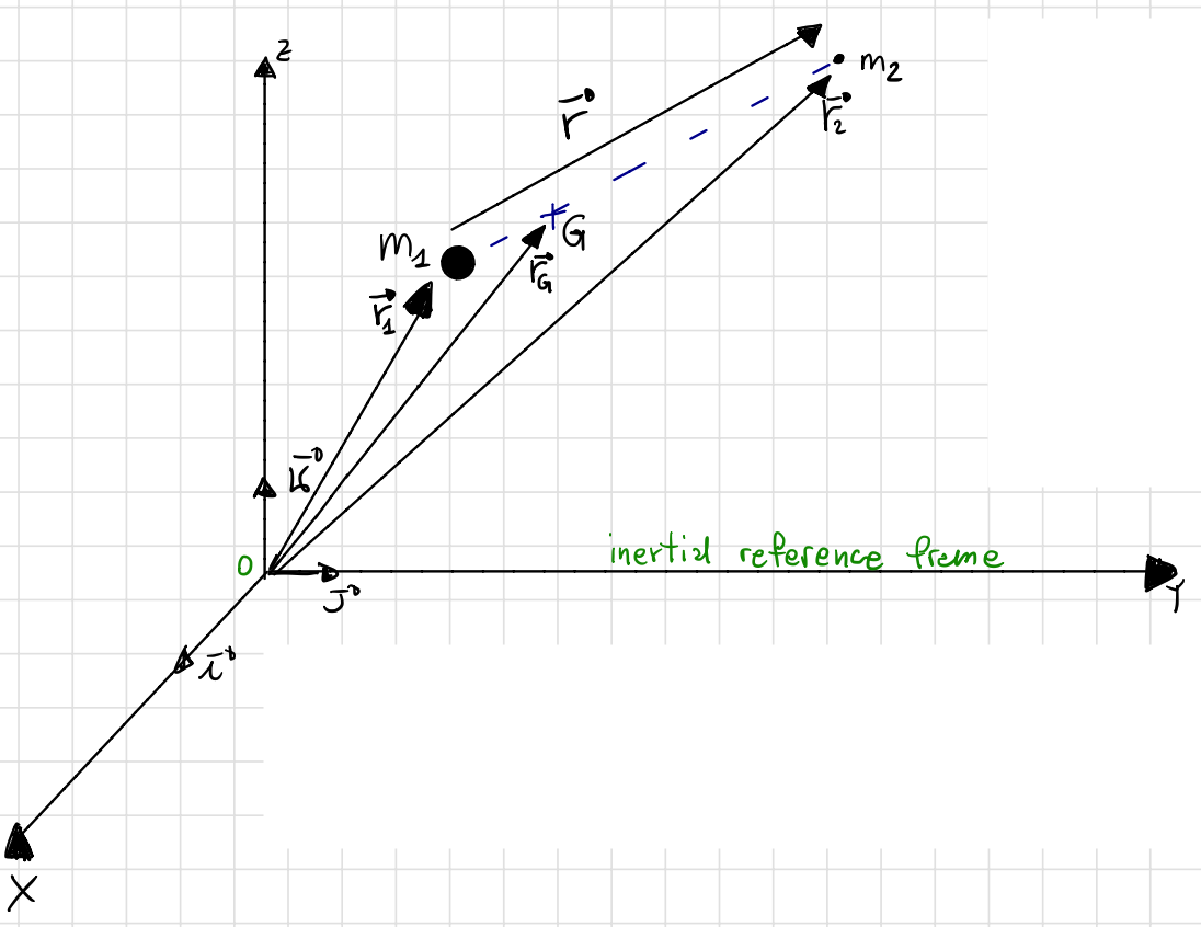
Fig. 1 The two-body dynamics of two particles \(m_1\) and \(m_2\) with position vectors \({\bf{r}}_1\) and \({\bf{r}}_2\) respectively.

Center of Mass ( G ) and its derivatives

The center of mass \({\bf{r}}_G\) of the system is given by:

(20)\[\begin{split}{\bf{r}}_G &= \frac{m_1 {\bf{r}}_1 + m_2 {\bf{r}}_2}{m_1 + m_2}\\ \Rightarrow {\bf{v}}_G &= \frac{m_1 {\dot{\bf{r}}}_1 + m_2 {\dot{\bf{r}}}_2}{m_1 + m_2}\\ \Rightarrow {\bf{a}}_G &= \frac{m_1 {\ddot{\bf{r}}}_1 + m_2 {\ddot{\bf{r}}}_2}{m_1 + m_2}\\\end{split}\]

Gravitational Force

Gravitational forces exists due to the two masses \(m_1\) and \(m_2\) and they act on each of the particles. These forces are shown in the Fig. 2 below as \({\bf{F}}_{12}\) and \({\bf{F}}_{21}\) acting on each of the particles.

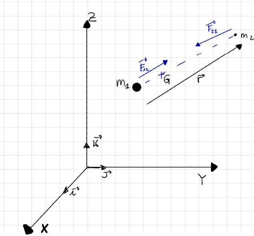
Fig. 2 Free-body diagram showing gravitational force in relative two-body dynamics of \(m_1\) and \(m_2\).

Here:

• \({\bf{F}}_{12}\) represents the force on \(m_1\) exerted by \(m_2\)’s gravitational attraction.

• \({\bf{F}}_{21}\) represents the force on \(m_2\) exerted by \(m_1\)’s gravitational attraction.

They are given by:

(21)\[\begin{split}\begin{aligned} {\bf{F}}_{12} &= \frac{G m_1 m_2}{r^2} \hat{\bf{r}} = \frac{G m_1 m_2}{r^3} {\bf{r}} \\ {\bf{F}}_{21} &= -\frac{G m_1 m_2}{r^2} \hat{\bf{r}} = -\frac{G m_1 m_2}{r^3} {\bf{r}} \end{aligned}\end{split}\]

\(G = 6.672 \times 10^{-11} \ \text{kg}^{-1} \ \text{m}^3 \ \text{s}^{-2}\) (Universal gravitational constant). Note that in (21), \({\bf{r}}\) is relative position vector and can be used to rewrite a position vector along itself as:

\[ \hat{\bf{r}} = \frac{{\bf{r}}}{|\bf{r}|}. \]

Newton’s Second Law (\({\bf F} = m{\bf a}\)) for \(m_1\) is:

(22)\[m_1 \ddot{\bf{r}}_1 = {\bf{F}}_{12}\]

Newton’s Second Law for \(m_2\) is:

(23)\[m_2 \ddot{\bf{r}}_2 = {\bf{F}}_{21}\]

Adding equations (22) and (23), then substituting for \({\bf{F}}_{12}\) and \({\bf{F}}_{21}\) from (21) gives us:

(24)\[\begin{split}m_1 \ddot{\bf{r}}_1 + m_2 \ddot{\bf{r}}_2 &= {\bf{F}}_{12} + {\bf{F}}_{21}\\ m_1 \ddot{\bf{r}}_1 + m_2 \ddot{\bf{r}}_2 &= \frac{G m_1 m_2 {\bf{r}}}{r^3} - \frac{G m_1 m_2 {\bf{r}}}{r^3}\\ m_1 \ddot{\bf{r}}_1 + m_2 \ddot{\bf{r}}_2 &= 0 \end{split}\]

Noting that the LHS of (24) is the same as the numerator of the acceleration of the center of mass (see the third of equations (20)), we have:

(25)\[\begin{split}\ddot{\bf{r}}_G &= 0\\ \dot{\bf{r}}_G &= \text{constant}\end{split}\]

This implies that \(G\) is inertially fixed (i.e., not accelerating) and so it can be chosen as the origin of another inertial reference frame (this is diffefrent from the one written in green in Fig. 1 above). It can also be easily inferred that the absolute (or inertial) velcoity of \(G\) is constant as the acceleration is zero. This is shown below and is consistent with the equation pair (25) above.

(26)\[\begin{split}\bf{a}_G &= 0\\ \bf{v}_G &= \text{constant}\end{split}\]

Two-Body Relative Dynamics

To study the relative motion of the two particles, we can subtract the equations of motion for each of the particles as given by (22) and (23). Before doing that, let’s rewrite the equations of motion for each of the particles. Newton’s Second Law for \(m_2\) is given by (23)

(27)\[m_2 \ddot{\bf{r}}_2 = {\bf{F}}_{21} = - \frac{G m_1 m_2 {\bf{r}}}{r^3} \rightarrow \ddot{\bf{r}}_2 = - \frac{G m_1 {\bf{r}}}{r^3}\]

Similarly, Newton’s Second Law for \(m_1\), given by (22), can be rewritten as:

(28)\[m_1 \ddot{\bf{r}}_1 = {\bf{F}}_{12} = \frac{G m_1 m_2 {\bf{r}}}{r^3} \rightarrow \ddot{\bf{r}}_1 = \frac{G m_2 {\bf{r}}}{r^3}\]

Subtracting (27) from (28) gives us the equation of motion for the relative motion of \(m_2\) with respect to \(m_1\) (the resulting is (31)):

(29)\[\ddot{\bf{r}} = \ddot{\bf{r}}_2 - \ddot{\bf{r}}_1 = - \frac{G m_1 {\bf{r}}}{r^3} - \frac{G m_2 {\bf{r}}}{r^3} = - \frac{G (m_1 + m_2) {\bf{r}}}{r^3}\]

(30)\[\ddot{\bf{r}} = - \frac{G (m_1 + m_2)}{r^3} {\bf{r}}\]

Attention

Equation (30) is written more commonly in shorthand using \(\mu\), the gravitational parameter, and gives the relative two-body dynamics equation

(31)\[\ddot{\bf{r}} = - \frac{\mu}{r^3}{\bf{r}}\]

Implications of this equation of motion

In most common cases of study/in this text, \(m_1 \gg m_2\). For example, \(m_1\) is \(m_\oplus = 5.974 \times 10^{24} \ \text{kg}\) and \(m_2\) is a spacecraft, \(m_2 \approx 1000 \ \text{kg}\)

(32)\[{\bf{r}}_G \approx {\bf{r}}_1\]

(33)\[\mu \approx G m_1\]

This is referred to as a restricted two-body problem.

Equation (30) is a vector ordinary differential equation (ODE). As we are studying the motion in a 3-dimensional coordinate system, this can also be written as a system of 3 scalar second-order ODE. However, they can be further reduced to a system of 6 first-order scalar ODEs or, as shown below, 2 first-order scalar ODEs:

(34)\[\bf{\dot r} = \bf{v}\]

(35)\[\bf{\dot v} = -\frac{\mu}{r^3}\bf{r}\]

Note

To solve a differential equation , we must know the intial values of the parameter we are solving for

To solve this system as a set of scalar ODEs, we need 6 initial conditions with \(\bf{r_0}\) and \(\bf{v_0}\):

(36)\[{\bf{r}} (t_0) = \bf{r_0}\]

(37)\[{\bf{v}} (t_0) = \bf{v_0}\]

This system of equations can admit, at maximum, 6 independent integrals of motion

Note

An Integral of Motion is a function, say \(f({\bf{r}} , {\bf{v}} , t )\), that is constant for all times, \(t\).

(38)\[f({\bf{r}} , {\bf{v}} , t) = constant\]

The value of the constant is determined by the intial conditions that permit us to solve the ODEs. An integral of motion reduces the degrees-of-freedom of a problem.

Specific Angular Momentum

The relative angular momentum of \(m_2\) with respect \(m_1\) is

(39)\[\begin{split}{\bf H}_{2/1} = {\bf{r}}\times( m_2 {\bf{v}})\\ \Rightarrow {\bf H}_{2/1} = {\bf{r}}\times( m_2 {\bf{\dot r}})\end{split}\]

and specific angular momentum is obtained by dividing a body’s relative angular moemntum from its mass. In case of \(m_2\), the specific angular momentum is givent by

(40)\[\begin{split}{\bf{h}} &= \frac{{\bf H}_{2/1}} {m_2}\\ {\bf{h}} &= \bf{r} \times \bf{v} {\bf{h}} &= \bf{r} \times \bf{\dot r}\end{split}\]

The time derivative of \(\bf{h}\) is

(41)\[\begin{split}\frac{\mathrm{d}\bf{h}}{\mathrm{d}t} &=\frac{\mathrm{d}}{\mathrm{d}t}(\bf{r}\times\bf{\dot r})\\ \Rightarrow \frac{d\bf{h}}{\mathrm{d}t} &= \bf{\dot r}\times\bf{\dot r} + \bf{r}\times\bf{\ddot r}\\ \Rightarrow \frac{\mathrm{d}\bf{h}}{\mathrm{d}t} &= \bf{r}\times\bf{\ddot r}\end{split}\]

From the two-body dynamics equation (30), we can rewrite the RHS of (41) as:

(42)\[\begin{split}\Rightarrow \frac{\mathrm{d}\bf{h}}{\mathrm{d}t} &=\bf{r}\times-\frac{\mu}{r^3}\bf{r}\\ \Rightarrow \frac{\mathrm{d}\bf{h}}{\mathrm{d}t} &=0\end{split}\]

which tells us that specific angular momentum is a constant.

(43)\[{\bf h} = \textbf{constant}\]

The implication of constant specific angular momentum is that:

1. \({\bf{h}}({\bf{r}} , {\bf{\dot r}} , t)\) = \(\textbf{constant}\), which means that \(\bf{h}\) is an integral of motion.

2. The 3 scalar components of \(\bf h\) are also constants. Or, in mathetmical terminology, we write:

\[\begin{split}h_x({\bf{r}} , {\bf{\dot r}} , t) &= \textit{constant}\\ h_y({\bf{r}} , {\bf{\dot r}} , t) &= \textit{constant}\\ h_z({\bf{r}} , {\bf{\dot r}} , t) &= \textit{constant}\end{split}\]

Kepler’s Second Law

We infer Kepler’s second law based on consequences relating to the nature of constant specific angular momentum vector; specifically, we examine the direction and then the magnitude of the specific angular momentum.

Direction

Firstly, from

(44)\[\bf{h} = \bf{r}\times\bf{v}\]

we can determine that

(45)\[\bf{h}\perp\bf{r}, \bf{v} \]

Recall: why is \(\bf{h}\) prependicular to both \(\bf{r}\) and \(\bf{v}\)?

This is because the result of cross-product between two vectors is a third vector that is orthogonal to both vectors.

Thus, \(\bf{r}\) and \(\bf{v}\) are at all times lie in a plane that is perpendicular to \(\bf{h}\). This also means that the motion is planar.

Magnitude

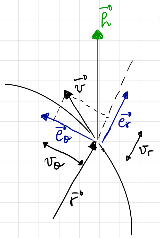
Fig. 3 Magnitude and direction of specific angular momentum.

Polar coordinates

\({\bf e}_r\) is directled along the position vector \(\bf r\) and \({\bf e}_{\theta}\) is perpendicular to it. The pair of vectors lie in the plane of the paper (or screen, in this case) and a third unit vector is directed orthogonal to them. This set of unit vectors make up a polar coordinate system.

From Fig. 3, we can make use of the polar coordinates \({\bf e}_r\) and \({\bf e}_{\theta}\) to write the component form of specific angular momentum.

(46)\[\begin{split}{\bf h} &= {\bf r}\times\bf{v}\\ \Rightarrow {\bf h} &= {\bf r}\times(v_{r} {\bf e}_r + v_{\theta}{\bf e}_{\theta})\\ \Rightarrow {\bf h} &={\bf r}\times(v_r{\bf e}_{r}) + {\bf r}\times(v_\theta {\bf e}_{\theta})\end{split}\]

where we have written the velocity vector \(\bf{v}\) as a sum of its components along the radial and angular directions:

(47)\[{\bf v} = v_r \bf{e}_r + v_\theta \bf{e}_\theta\]

noting that \(v_r\) is the scalar component of the velocity along the radial direction and \(v_\theta\) is the scalar component of the velocity along the angular direction.

The first term on the RHS of the last of Equations (46) is zero because \(\bf{r}\) and \(\bf{v_r}\) are parallel; thus the second term is the only term remaining. As a result, this must be directed along the angular momentum vector \(\bf{h}\). It can also be written along a unit vector along the direction of \(\bf{h}\), called \(\bf{\hat{h}}\):

(48)\[\begin{split}{\bf h} &=rv_\theta{\hat{\bf{h}}}\\ \Rightarrow {\bf h} &= h {\hat{\bf{h}}}\end{split}\]

From Equation (43), we know that the angular momentum \(\bf h\) is constant, which further implies that \(r v_\theta\) is constant. Or, in other words, the scalar \(h\) denoting the magnitude of the specific angular momentum is a constant.

(49)\[h = rv_\theta = \textit{constant}\]

Areal velocity and Kepler’s Second Law

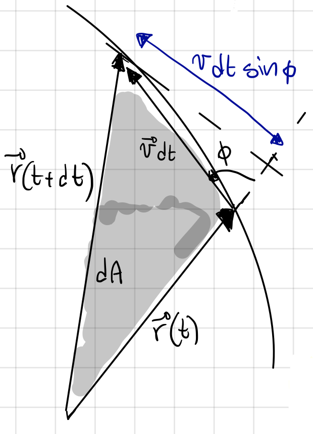
Fig. 4 The grey area is swept by the positon vector in a small interval of time \(\mathrm{d}t\).

From Fig. 4, we can write the infinitesimal area \(\mathrm{d}A\) swept by \(\bf r\) as

(50)\[\mathrm{d}A = \frac{1}{2}r\, v\, \mathrm{d}t\sin(\phi)\]

wihch can be further rewritten

(51)\[\begin{split}\frac{\mathrm{d}A}{\mathrm{d}t} &= \frac{1}{2}r\, v\, \sin(\phi)\\ \Rightarrow \frac{\mathrm{d}A}{\mathrm{d}t}&= \frac{1}{2}r\, v_\theta \end{split}\]

or

(52)\[\frac{\mathrm{d}A}{\mathrm{d}t}=\frac{1}{2}h = constant\]

This is essentially giving us Kepler’s Second Law, which tells us that areal velocity is constant. In other words, it tells us that equal areas are swept in equal intervals of time along the orbit in a body whose dynamics are governed by the simple two-body system described by Equation (31).

Two-body Dynamics in Polar Coordinates

If the motion is planar, we can use polar coordinates to fully describe it. Consider a situation where this planar motion lies in the x-y plane shown in Fig. 5.

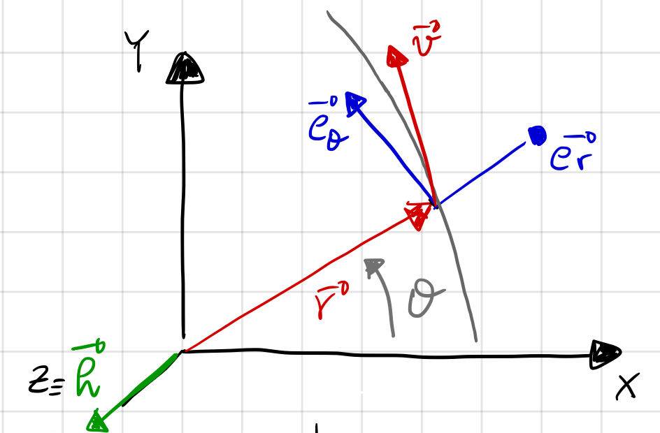
Fig. 5 Polar coordinate system (in blue) to study the two-body problem.

Using polar coordinates shown in Fig. 5, we can see that \(\bf{r} = r\bf{e_r}\). Thus

(53)\[\frac{d\bf{r}}{dt} = {\bf v} = {\dot r}{ \bf e}_r + {r}{\dot \theta}{\bf e}_\theta \]

which allows us to write

(54)\[\begin{split}{\bf h} &= {\bf r} \times {\bf v}\\ &=r {\bf e}_r \times ({\dot r} {\bf e}_r + {r} \dot \theta {\bf e}_\theta)\end{split}\]

or

(55)\[\begin{split} {\bf h} &= r^2\dot \theta \hat{\bf{k}}\\ &= rv_\theta \hat{\bf{k}} = constant\end{split}\]

where \(\hat{\bf{k}}\) is a unit vector orthogonal to \({\bf e}_r\) and \({\bf e}_\theta\). Further, we can substitute for \(h\) from (55) into to (52), which gives

(56)\[\begin{split}\frac{\mathrm{d}A}{\mathrm{d}t} &= \frac{1}{2}h\\ \frac{\mathrm{d}A}{\mathrm{d}t} &= \frac{1}{2}r^2\dot \theta\end{split}\]

Taking the second derivatibe of \(\bf r\) using (53), we get

(57)\[{\frac{d^2\bf{r}}{\mathrm{d}t^2}} = \ddot{\bf r} = ({\ddot r} - r\dot\theta^2) {\bf{e_r}} + (r\ddot \theta+2\dot r\dot \theta) {\bf{e_\theta}}.\]

We can also write the RHS of (31) in polar coordinates as

(58)\[\frac{-\mu}{r^2}\bf{e_r}\]

which upon comparing to (57) gives the following two scalar ODEs along the \({\bf e}_r\) and \({\bf e}_\theta\) directions, respectively:

(59)\[\begin{split}{\ddot r} - r\dot \theta^2 &= \frac{-\mu}{r^2}\\ r\ddot \theta + 2{\dot r}\dot \theta &= 0\end{split}\]

Note that the second of Equations (59) can also obtained from differentiating the specific angular momentum

(60)\[\begin{split}\frac{d}{dt}(h) &= \frac{d}{dt}(r^2\dot \theta)\\ \Rightarrow &=2r{\dot r}\dot \theta+r^2\ddot \theta\\ \Rightarrow &=r(r\ddot \theta+2{\dot r}\dot \theta)\\ \Rightarrow &=0\end{split}\]

In other words, the second of Equations (59) is equivalent to \(h = constant\).

Conservation of Specific Orbital Energy: \(E\)

In this section we show that specific energies of orbits are constant, under two-body dynamics. To do so, we begin by computing dot product between \(\bf{\dot r}\) and both sides of the two-body dynamics equation (Equation (31)):

(61)\[{\dot{\bf r}} \cdot \ddot{\bf r} = \frac{-\mu}{r^2} \hat{\bf r} \cdot{\dot{\bf r}}\]

Further, we note the following

(62)\[\frac{d}{dt}(\frac{1}{2}v^2)=\frac{1}{2}\frac{d}{dt}(\bf{\dot r\cdot\dot r}).\]

The derivative on the RHS of Equation (62) also yields

(63)\[\frac{1}{2}{\ddot{\bf r}} {\cdot\dot{\bf r}} + \frac{1}{2}{\dot{\bf r}} \cdot {\ddot{\bf r}} = \dot{\bf r} \cdot {\ddot {\bf r}}.\]

This tells us that the term on LHS of Equation (61) can be written as shown below

(64)\[\dot{\bf r} \cdot \ddot{\bf r} = \frac{d}{dt}(\frac{1}{2}v^2)\]

Notice that this is the derivative of a term that resembles kinetic energy (but lacking a term for mass).

Note

In polar coordinates \(v^2={v_r}^2+{v_\theta}^2={\dot r}^2+r^2\dot \theta^2\)

Further,

Using the chain rule, we have written

\[\frac{d}{dt} \Bigl( \frac{\mu}{r} \Bigl) = \frac{\partial}{\partial r} \Bigl( \frac{\mu}{r} \Bigr) \frac{dr}{dt}\]

This means we first differentiate \(\frac{\mu}{r}\) with respect to \(r\), and then multiply by how \(r\) changes with time.

(65)\[\frac{d}{dt} \Bigl( \frac{\mu}{r} \Bigl) = \frac{\partial}{\partial r} \Bigl( \frac{\mu}{r} \Bigr) \frac{dr}{dt} = -\frac{\mu}{r^2}{\dot r}\]

Noting the above and observing that \({\bf \hat{r}} \cdot {\dot{\bf r}} = v_r = \dot r\) , the term on the RHS of Equation (61) is rewritten as below

(66)\[-\frac{\mu}{r^2}{\bf{\hat{r}}}{\cdot\bf{\dot r}} = \frac{\mu}{r^2}\dot r = \frac{d}{dt}\Bigl(\frac{\mu}{r} \Bigr)\]

Important

Notice that the term on the RHS of Equation (61) has been recomputed as the derivative of the potential of the gravitational force.

Substituting the derivatives of kinetic Energy (64) and potential of gravitationl force (66) into (61) gives

(67)\[\frac{d}{dt}(\frac{1}{2}v^2-\frac{\mu}{r})=0\]

from which follows the Conservation of Specific Orbital Energy (68):

(68)\[\frac{1}{2}v^2-\frac{\mu}{r} = constant\]

where \(E\) the specific orbital energy is given by

(69)\[E = \frac{1}{2}v^2-\frac{\mu}{r}\]

Admissible Orbital Radius

Starting from Equation (69), we can rewrite \(E\) as

(70)\[\begin{split}E &= \frac{1}{2}v^2- \Bigl(\frac{\mu}{r}\Bigr)\\ \Rightarrow E &= \frac{1}{2}{\dot r}^2+\frac{1}{2}r^2\dot \theta-\Bigl(\frac{\mu}{r}\Bigr)\\ \Rightarrow E &= \frac{1}{2}{\dot r}^2+\Bigl(\frac{1}{2}\frac{h^2}{r^2}-\frac{\mu}{r}\Bigr)\end{split}\]

Focusing on the terms within the brackets on the RHS of Equation (70), we can define a few terms:

• the entire collection of terms \(\frac{1}{2}\frac{h^2}{r^2}-\frac{\mu}{r}\) is called the effective potential and denoted by \(\phi_{eff}(r)\).

• the first of these terms, \(\frac{1}{2}\frac{h^2}{r^2}\), is known as the potential of the centrifugal force; and

• the second of these terms, \(-\frac{\mu}{r}\), is referred to as the potential of the gravitational force.

Fig. 6 shows a qualitative depiction of the contribution of each of these terms to the effective potential separately and how their sum shapes the effective potential.

Fig. 6 Qualitative depiction of \(\phi_{eff}(r)\) and its contributions from the two terms in brackets on the RHS of Equation (70).

The effective potential can take positive or negative values over a range of values of \(r\) given its definition.

Now, Equation (70) can be written as

(71)\[E = \frac{1}{2}{\dot r}^2 + \phi_{eff}(r) = constant\]

From this equation, we can infer that:

• the kinetic energy term \(\frac{1}{2}{\dot r}^2 \geq 0\).

• therefore \(E\geq\phi_{eff}(r)\).

Thus motion is only possible for those values of \(r\) such that \(E\geq\phi_{eff}\).

Fig. 7 is a qualitative depiction of the \(\phi_{eff}\) as a function of \(r\):

Fig. 7 \(\phi_{eff}\) as a function of \(r\).

This is a more detailed depiction of Fig. 6, which also shows the constant specific energy \(E\) as a blue horizontal line. Indeed, as \(E\) is constant, it can easily be computed from the initial conditions of the system. \(E\) can take on various values, each corresponding to a different orbit:

• When \(E<0\), the motion occurs between \(r_{min}\) and \(r_{max}\) telling us that the motion is bounded. More specifically, it is an elliptical orbit; this condition is shown clearly in Fig. 7.

• When \(E\geq0\) the motion is unbounded; this case is shown in the right side of Fig. 8.

• For \(E=\min{\phi(r)}\), we get the condition that \(r_{min}=r_{max}\) resulting in a circular orbit. This case is shown in the left side ofFig. 8.

Fig. 8 On the left plot, we see that \(E\) aligns with the minimum value of \(\phi_{eff}\) at \(r_{min}\) and \(r_{max}\). On the right plot, we see that for \(E\geq0\), the motion is unbounded.

Key points

Key takeaways from the discussion so far are that when we are given the initial position \(\bf{r_0}\) and velocity \(\bf{v_0}\) we can compute:

1. Specific angular momentum \(\bf{h}\) as shown below:

(72)\[{\bf h}={\bf h_0}=constant\]

which is orthogonal to the orbital plane. The intial values also tells us that the constant areal velocity is \(r_0^2\dot \theta_0\).

2. Specific orbital energy \(E\) as shown below

(73)\[E_0=\frac{1}{2}v_0^2 - \frac{\mu}{r_0}\]

where \(E_0\) is the specific orbital energy at computed from the initial conditions. If \(E<0\), we have a bounded orbit but if \(E\geq0\) we have unbounded motion.

3. Compute the minimum or maximum values of \(r\) when \(\phi_{eff}=E=E_0\).