Problem Set 2

Problem Set 2#

Earth data $$ R^{Equator} = 6384 km $$ R^{Pole} = 6353 km $$ \mu = 3.986 \times 10^5 km^3s^{-2} $$

Question 1#

A remote sensing satellite is in a polar orbit with its line of apsides on the equator. The perigee of the orbit is at altitude of $620$ $km$ and the eccentricity of the orbit is $e = 0.04$. Calculate the semi-major axis of this orbit and show that the altitude at apogee is approximately $1200$ $km$.

Solution 1#

We are told that $e$, the eccentricity of the orbit, is 0.04. And that the altitude at perigee, denoted by $h_p$, is $620$ $km$. We are asked to determine $a$ (semi-major axis of the orbit) and the altitude at perigee, which we shall denote as $h_p$. For this purpose, we will also create the following symobls:

$r_p$ is the satellite’s perigee;
$r_a$ is the satellite’s apogee.

For an elliptic orbit, the satellite’s perigee point is given by $$ r_p = a(1-e) \tag{2.1} $$ or $$ a = \frac{r_p}{1-e} \tag{2.2} $$. By rewriting $r_p$ as a sum of $R^{Equator}$ and $h_p$, we can rewrite the above equation as $$ a = \frac{R^{Equator} + h_p}{1-e}. \tag{2.3} $$ Then, we substitute for the above to get that $a = 7295.83km$.

It is easier and clearer to do the above work with a computer; in this module, we make use of the Python programming language.

# Your coded answers here (and create more Code cells if you wish to)
R_Equator = 6384
h_p = 620
e = 0.04
r_p = R_Equator + h_p
a = (r_p)/(1 - e)
a

7295.833333333334

The altitude at apogee, $h_a$, is given by $$ h_a = r_a - R^{Equator} \tag{2.4} $$ or $$ h_a = a(1+e) - R^{Equator} \tag{2.5} $$ which gives $h_a = 1203.66$.

h_a = a*(1+e) - R_Equator
h_a

1203.6666666666679

Question 2#

The satellite carries a camera with a field of view of $26^o$. The camera has a CCD array of $1000$ pixels. Compute the resolution per pixel of this camera at perigee and apogee.

Solution 2#

The resolution, which has units of $m/ pixel$, is a function of a parameter called swath; a schematic to understand this is sketched out below.

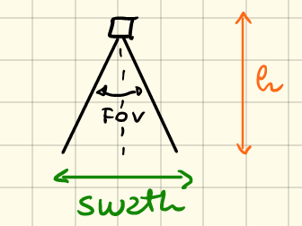
In the above $FoV$ is the field of view of the imaging system (i.e., CCD array), which is in radians. Form this, we can see that swath, $s$, can be calucalted easily. For example, the swath from perigee, $s_p$, $$ s_p = 2*h_p*\tan(FoV/2). \tag{2.6} $$ You should be able to justify to yourselves why the above formula is correct based on fundamental trigonometry. Once $s_p$ is known, we can calculate the resolution from perigee, $r_p$: $$ r_p = \frac{s_p}{\textrm{number of pixels}} \tag{2.7} $$ You can repeat this process for to determine $r_a$, (where the subscript $a$ corresponds to apogee). It is easier and clearer to do the above work with a computer; in this module, we make use of the Python programming language. To aid our computations, Python has a mathz library from which we can import the tanandpi` functions for accurate calculations.

# Your coded answers here (and create more Code cells if you wish to)
from math import tan, pi
pixelCount = 1000
field_of_view_in_degrees = 26
field_of_view_in_radians = field_of_view_in_degrees*pi/180

swath_from_perigee = 2*h_p*tan(field_of_view_in_radians/2)
swath_from_apogee = 2*h_a*tan(field_of_view_in_radians/2)

resolution_from_perigee = swath_from_perigee/pixelCount
resolution_from_apogee = swath_from_apogee/pixelCount
("The resolutions from perigeed and apogee, respectively, in km/pixel are", resolution_from_perigee, resolution_from_apogee)

('The resolutions from perigeed and apogee, respectively, in km/pixel are',
 0.28627655699569826,
 0.5557766921029395)

Note that the handwritten solutions provide the solutions in the $m/pixel$.

Question 3#

Find the altitude of the satellite as it passes over the poles. For the camera onboard the satellite, compute the image resolution over the poles.

Solution 3#

We know that the general relationship to compute the satellite’s position, $r$, is $$ r = \frac{a(1-e^2)}{1+e\cos(\theta)}. \tag{2.8} $\theta = 90^o$ at the poles, so $$ r_{poles} = a(1-e^2). \tag{2.9} $$ The height at the poles is then given by $$ h_{poles} = p - r_{poles}. \tag{2.10} $$

We can then compute the resolution at the poles using a procedure identical to that shown in Solution 2 for the perigee and apogee. This is illustrated in Python code below.

# Your coded answers here (and create more Code cells if you wish to)
r_poles = a*(1-e**2)
Radius_of_Earth_at_poles = 6353
h_poles = r_poles - Radius_of_Earth_at_poles

swath_from_poles = 2*h_poles*tan(field_of_view_in_radians/2)
resolution_from_poles = swath_from_poles/pixelCount

print("The altitude at the poles in km is ", h_poles)
print("The resolution from the poles in km/pixel is", resolution_from_poles)

The altitude at the poles in km is  931.1599999999999
The resolution from the poles in km/pixel is 0.4299504496969586

Question 4#

Calculate the velocity of this spacecraft at perigee, and the angular velocity. Neglecting the eccentricity of the orbit and taking the Earth as a sphere, how long will it take for the spacecraft to disappear over the horizon of an observer directly below the perigee point?

Solution 4#

Part a: Compute $v_p$#

We make us of the vis-viva equation as shown below, $$ \frac{1}{2}v_p^2 - \frac{\mu}{r_p} = -\frac{\mu}{2a}, \tag{2.11} $$ where the subscript $p$ indicates that the point of interest is the satellite's perigee. We can then solve for $v_p$ as $$ v_p = \sqrt{\frac{2\mu}{r_p} -\frac{\mu}{a}} \tag{2.12} $$ which, upon substituting for the known terms, give us $v_p = 7.69km/s$.

Part b: Compute $\dot\theta$#

Further, at perigee, we know that there is no radial component to velocity; so, considering the velcoity vector $$ {\bf v} = \dot r {\bf \hat e}_r + r \dot \theta{\bf \hat e}_\theta. \tag{2.13} $$, we can write the following scalar equations, $$ \dot r = 0 \tag{2.14} $$ and $$ v_p = r \dot\theta. \tag{2.15} $$

The angular velocity at perigee can then be computed by rewriting Equation $(2.15)$ as $$ \dot\theta = \frac{v_p}{r_p} \tag{2.16} $$ which gives $\dot\theta = 1.09 \times 10^{-3}rad/s$.

Part c: Computing the time for which an observer below perigee can see the satellite#

Note that if the eccenticity is ignored, then the satellite is on a circular orbit; this means that it has the same altitude at any orbit (or $r=r_p$ at all points on the orbit). To determine the time of disappearance, we first need to know the half-angle at which the satellite is no longer visible to the observer on the surface of the Earth and below perigee; this is shown as $\alpha$ in the schematic below.

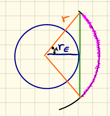
\[ \alpha = \cos^{-1}\bigg(\frac{R_{Equator}}{r_p}\bigg) \]

Once $\alpha$ is known, we can compute the duration of observation of the satellite by this oberver, $t_{obsv}$, by $$ t_{obsv} = 2\frac{\alpha}{\dot\theta}. \tag{2.17} $$ Can you explain to yourselves why we there is a doubling term (i.e. scaling factor of $2$) in the RHS of Equation $(2.17)$?

We present the computation with Python below’; sqrt helps in computing the square-root and acos helps in computing the inverse cosine value of a function (i.e. $\cos^{-1}$).

# Your coded answers here (and create more Code cells if you wish to)
from math import sqrt, acos
# Part a: Compute $v_p$
mu_Earth = 3.986 * 10**5
v_p = sqrt(2*mu_Earth /r_p - mu_Earth/a)
print("Velocity at perigee is ", v_p, "km/s")

# Part b: Compute $\dot\theta$
angular_velocity = v_p/r_p
print("Angular velocity at perigee is", angular_velocity, "rad/s")

# Part c: Computing the time for which an observer below perigee can see the satellite
alpha = acos(R_Equator/r_p)
t = 2 * alpha/angular_velocity
print("The satellite can be observed by the obersver for", t , "s")

Velocity at perigee is  7.693292560947274 km/s
Angular velocity at perigee is 0.001098414129204351 rad/s
The satellite can be observed by the obersver for 771.8957207955966 s