Determining Orbital Paths

Determining Orbital Paths#

Prepared by: Noah Leigh, Ilanthiraiyan Sivagnanamoorthy, and Angadh Nanjangud

In this lecture we aim to cover the following topics:

Orbital Elements from Position and Velocity Vectors
Rotation Matrix (Direction Cosines Matrix)
ECI to Perifocal Frame
Ephemeris: Position and Velocity Vector as Function of Time

Orbital Elements from Position and Velocity Vectors#

Orbital Parameters

Calculate the semi-major axis $a$ from the Vis-Viva equation (84):

\[a = \frac{\mu}{2\epsilon} \]

Compute the eccentricity $e$ (76) from:

\[\mathbf{e} = \frac{\mathbf{v} \times \mathbf{h}}{\mu} - \frac{\mathbf{r}}{|\mathbf{r}|}\]

Compute the inclination $i$ from:

(133)#\[\mathbf{h_z}=\mathbf{h}\cos \left( i \right)\]

Compute the right ascension of the ascending node $\Omega$ from:

(134)#\[\cos \left(\Omega\right)= \frac{n_y}{|\mathbf{n}|}\]

Determine the correct quadrant:
- If $n_y \geq 0$, then $\Omega \in [0, 180^\circ]$
- If $n_y < 0$, then $\Omega = 360^\circ - \cos^{-1} \left( \frac{n_x}{|\mathbf{n}|} \right)$

Compute the argument of perigee $\omega$ from:

(135)#\[\cos \left(\omega\right) = \frac{\mathbf{n} \cdot \mathbf{e}}{|\mathbf{n}| |\mathbf{e}|}\]

Determine the correct quadrant:
- If $e_z \geq 0$, then $\omega \in [0, 180^\circ]$
- If $e_z < 0$, then $\omega = 360^\circ - \cos^{-1}\left(\frac{\mathbf{n} \cdot \mathbf{e}}{|\mathbf{n}||\mathbf{e}|}\right)$

Compute the true anomaly $\theta$ from:

(136)#\[\mathbf{r}\cdot\mathbf{e} = |\mathbf{r}||\mathbf{e}|\cos \left( \theta \right)\]

Determine the correct quadrant: Need to calculate $v_r = \mathbf{v}\cdot\hat{r}$
- If $v_r \geq 0, \theta = \cos^{-1}\left(\frac{\mathbf{r}\cdot\mathbf{e}}{|\mathbf{r}||\mathbf{e}|}\right)$
- If $v_r < 0, \theta = 360^\circ - \cos^{-1}\left(\frac{\mathbf{r} \cdot \mathbf{e}} {|\mathbf{e}||\mathbf{r}|}\right)$

Note: Orbital parameters can be singular in certain conditions!

Rotation Matrix (Direction Cosines Matrix)#

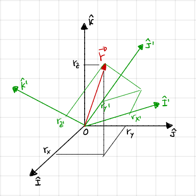
../../_images/reference_frames_L6.png — Fig. 10 Shows the two different reference frames, before transformation in black and after in green.#

Let’s define the unit vectors of two frames:

In the original frame: $\left(\mathbf{ \hat{I}, \hat{J}, \hat{K} }\right)$
In the transformed frame: $\left( \mathbf{\hat{I}', \hat{J}', \hat{K}'} \right)$

We want to express a vector r in two frames:

In the original frame: $\mathbf{r} = (\mathbf{r_x, r_y, r_z})$
In the transformed frame: $\mathbf{r'} = \left(\mathbf{r'_x, r'_y, r'_z}\right)$

Matrix Transformation:#

The transformation from the original frame to the new frame can be written as:

\[\mathbf{r'} = A\mathbf{r}\]

\[\begin{split} A = \begin{bmatrix} \mathbf{I'}\cdot\mathbf{I} & \mathbf{I'}\cdot\mathbf{J} & \mathbf{I'}\cdot\mathbf{K} \\ \mathbf{J'}\cdot\mathbf{I} & \mathbf{J'}\cdot\mathbf{J} & \mathbf{J'}\cdot\mathbf{K} \\ \mathbf{K'}\cdot\mathbf{I} & \mathbf{K'}\cdot\mathbf{J} & \mathbf{K'}\cdot\mathbf{K} \end{bmatrix} \end{split}\]

Each row of A contains the components of $\mathbf{I',J',K'}$ in the $\mathbf{I,J,K}$ reference frame. and vice versa for the columns.

Properties of the Rotation Matrix, $A$:#

The columns of $A$ contain the components of the unit vectors $\mathbf{I, J, K}$ in the transformed frame $\mathbf{I', J', K'}$.
The inverse transformation is given by:

\[ \mathbf{r} = A'\mathbf{r'} \]

Since $A$ is an orthogonal matrix, the inverse of $A$ is equal to its transpose:

\[ A' = A^T \]

This gives us the property:

\[ A^TA = I \]

Where $I$ is the identity matrix.

The norm of each row of $A = 1$ and the dot product between rows = 0 $\Rightarrow$ 6 constraints $\Rightarrow$ 9 elements - 6 constraints = 3 Degrees of Freedom.

Successive Rotations:#

If two successive rotations are performed, say $A_1$ and $A_2$, the net transformation matrix $A$ is the product of the two:

(137)#\[A = A_2A_1\]

This allows us to deal with complex rotations as a series of simpler rotations.

Rotation About a Single Axis:#

For rotation about the $\mathbf{I}$ $\left(\mathbf{\hat{I}}\equiv\mathbf{\hat{I}'}\right)$:

\[\begin{split} A_x(\alpha) = \begin{bmatrix} 1 & 0 & 0 \\ 0 & \cos(\alpha) & -\sin(\alpha) \\ 0 & \sin(\alpha) & \cos(\alpha) \end{bmatrix} \end{split}\]

$\mathbf{r'} = A_x(\alpha)\mathbf{r}$
Inverse - $\mathbf{r}=A_x(\alpha)^T\mathbf{r'}=A_x(-\alpha)\mathbf{r'}$
We can also associate an angular velocity to this rotation $\mathbf{\omega}=\alpha\mathbf{\hat{I}}$.

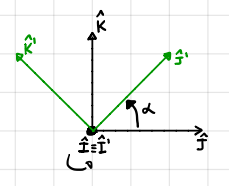
../../_images/rotation_about_I_L6.png — Fig. 11 Shows a rotation about x-axis, before transformation in black and after in green.#

For rotation about the $\mathbf{J}$ $\left(\mathbf{\hat{J}}\equiv\mathbf{\hat{J}'}\right)$:

\[\begin{split} A_y(\alpha) = \begin{bmatrix} \cos(\alpha) & 0 & \sin(\alpha) \\ 0 & 1 & 0 \\ -\sin(\alpha) & 0 & \cos(\alpha) \end{bmatrix} \end{split}\]

$\mathbf{r'} = A_y(\alpha)\mathbf{r}$
Inverse - $\mathbf{r}=A_y(\alpha)^T\mathbf{r'}=A_y(-\alpha)\mathbf{r'}$
We can also associate an angular velocity to this rotation $\mathbf{\omega}=\alpha\mathbf{\hat{J}}$.

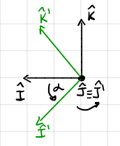
../../_images/rotation_about_J_L6.png — Fig. 12 Shows a rotation about y-axis, before transformation in black and after in green.#

For rotation about the $\mathbf{K}$ $\left(\mathbf{\hat{K}}\equiv\mathbf{\hat{K}'}\right)$:

\[\begin{split} A_z(\alpha) = \begin{bmatrix} \cos(\alpha) & -\sin(\alpha) & 0 \\ \sin(\alpha) & \cos(\alpha) & 0 \\ 0 & 0 & 1 \end{bmatrix} \end{split}\]

$\mathbf{r'} = A_z(\alpha)\mathbf{r}$
Inverse - $\mathbf{r}=A_z(\alpha)^T\mathbf{r'}=A_z(-\alpha)\mathbf{r'}$
We can also associate an angular velocity to this rotation $\mathbf{\omega}=\alpha\mathbf{\hat{K}}$.

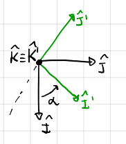
../../_images/rotation_about_K_L6.png — Fig. 13 Shows a rotation about z-axis, before transformation in black and after in green.#

ECI to Perifocal Frame#

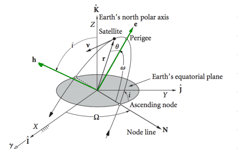
../../_images/ECI_L6.png — Fig. 14 Shows a satellite’s orbit described relative to Earth.#

Composition of Rotations:#

To rotate from the ECI (Earth-Centered Inertial) frame to the perifocal frame, we use three successive rotations:

Rotation by $\Omega$ about the z-axis: $$ A_z(\Omega) $$
Rotation by $i$ about the x-axis: $$ A_x(i) $$
Rotation by $\omega$ about the z-axis: $$ A_z(\omega) $$

The total transformation matrix, using successive rotations (137), is:

\[ A = A_z(\omega)A_x(i)A_z(\Omega) \]

with the respective direction matrices.

Transformation:
- Passage from the ECI frame to the perifocal frame is given by the composition of three rotations:
  
  (138)#\[\mathbf{r}_{perifocal} = A_z(\omega) A_x(i) A_z(\Omega) \mathbf{r}_{ECI}\]
Inverse Transformation:
- To transform from the perifocal frame back to ECI: $$ \mathbf{r}_{ECI}=\left[A_z(\omega)A_x(i)A_z(\Omega)\right]^T\mathbf{r}_{perifocal} =A^T_z(\Omega)A^T_x(i)A^T_z(\omega)\mathbf{r}_{perifocal} $$
(139)#\[\mathbf{r}_{ECI} = A_z(-\Omega) A_x(-i) A_z(-\omega) \mathbf{r}_{perifocal}\]

Ephemeris: Position and Velocity Vector as Function of Time#

Computing r and v at time, t, in ECI frame:

Compute the mean anomaly $M = n(t - t_0) + M_0$, ($n = \sqrt\frac{\mu}{a^3}$).
Solve Kepler’s equation $M = E - e\sin(E)$ for $E$ (the eccentric anomaly).
Find the true anomaly $\theta$ from:

(140)#\[\tan \left(\frac{\nu}{2}\right) = \sqrt{\frac{1+e}{1-e}} \tan \frac{E}{2}\]

Compute the position vector in the perifocal frame:

(141)#\[\begin{split}\mathbf{r}_{perifocal} = \frac{a(1 - e^2)}{1 + e \cos \left( \theta \right)} \begin{bmatrix} \cos (\theta) \\ \sin (\theta) \\ 0 \end{bmatrix}\end{split}\]

Compute the velocity vector in the perifocal frame:

(142)#\[\begin{split}\mathbf{v}_{perifocal} = \sqrt{\frac{\mu}{a(1 - e^2)}} \begin{bmatrix} -\sin (\theta) \\ e + \cos (\theta) \\ 0 \end{bmatrix}\end{split}\]

Transform the position and velocity vectors from the perifocal frame to the ECI frame using the inverse rotation matrices:

(143)#\[\mathbf{r}_{ECI} = A_3(\omega) A_2(i) A_1(\Omega) \mathbf{r}_{perifocal}\]

(144)#\[\mathbf{v}_{ECI} = A_3(\omega) A_2(i) A_1(\Omega) \mathbf{v}_{perifocal}\]

Note: $\sqrt {a(1-e^2)\mu} = h$, magnitude of the specific angular momentum.