Orbital Elements (Part 1)

Prepared by: Ilanthiraiyan Sivagnanamoorthy, Joost Hubbard, and Angadh Nanjangud

In this lecture we aim to cover the following topics:

1. Determination of Velocity Component

2. The Perifocal Frame

3. The ECI Reference Frame

4. Classical Orbital Parameters

Determination of Velocity Component

Recall from Equations (47) and (53) that, the polar coordinate form of the velocity vector can be written in various forms:

(128)\[\begin{split}\mathbf{v} &= \dot{\mathbf{r}}\\ &= v_r \mathbf{e}_r + v_\theta \mathbf{e}_\theta\\ &= \dot{r} \mathbf{e}_r + r \dot{\theta} \mathbf{e}_\theta\end{split}\]

Also recall that the equation of the orbit when given the semi-latus rectum (\(p\)), is given by Equation (83):

(129)\[r = \frac{p}{1 + e \cos\theta}\]

which can also be used to compute velocity (its magnitude). We do so using the chain rule, differentating \(r\) with respect to \(\theta\) and then multiplying by \(\dot \theta\):

\[\begin{split}\dot{r} &= \frac{dr}{dt}\\ &= \frac{\mathrm{d} r}{\mathrm{d} \theta} \frac{\mathrm{d} \theta}{\mathrm{d} t}\end{split}\]

To differentiate \(r\) with respect to \(\theta\), we define \(u \triangleq 1 + e \cos \theta\) which allows us to rewrite \(r\) as:

\[r = \frac{p}{u}\]

that allows us to again apply the chain rule:

(130)\[\frac{\mathrm{d} r}{\mathrm{d} \theta} = \frac{\mathrm{d} r}{\mathrm{d} u} \frac{\mathrm{d} u}{\mathrm{d} \theta}\]

where:

\[\frac{\mathrm{d} r}{\mathrm{d} u} = \frac{-p}{u^2}\]

and:

\[\frac{\mathrm{d} u}{\mathrm{d} \theta} = -e \sin\theta\]

thus giving us in Equation (130):

(131)\[\frac{\mathrm{d} r}{\mathrm{d} \theta} = \frac{p}{u^2} e \sin\theta\]

which, after substituting back \(u = 1 + e \cos \theta\), gives us:

(132)\[\frac{\mathrm{d} r}{\mathrm{d} \theta} = \frac{pe \sin \theta}{\left(1 + e \cos \theta\right)^2}\]

This results in the following derivative of Equation (129):

(133)\[\dot{r} = \frac{pe \sin \theta}{\left(1 + e \cos \theta\right)^2} \dot{\theta}\]

Substituting Equation (129) into (133) gives us:

(134)\[\dot{r} = \frac{r^2 \dot{\theta}}{p} e \sin \theta\]

which, given \(h = r^2\dot\theta\) and \(p = h^2/\mu\), can be expressed as:

(135)\[\dot{r} = \frac{\mu}{h} e \sin \theta\]

Expressions for \(v_r\) and \(v_\theta\)

From Equation (128), the radial component of velocity is simply \(\dot r\). So:

(136)\[v_r = \dot{r} = \frac{\mu}{h} e \sin \theta\]

Similarly, the tangential component is simply \(r \dot{\theta}\) and since \(h = r^2 \dot{\theta}\), we get:

(137)\[v_\theta = r \dot{\theta} = \frac{h}{r} = \frac{h \left(1 + e \cos \theta\right)}{h^2 / \mu} = \frac{\mu}{h} \left(1 + e \cos \theta\right)\]

Important

These derivations are valid for all \(e\), not only for ellipses.

Flight Path Angle

Using the expressions for \(v_r\) and \(v_\theta\) derived above, we can define the flight path angle, denoted by \(\gamma\), which is shown in the schematic below:

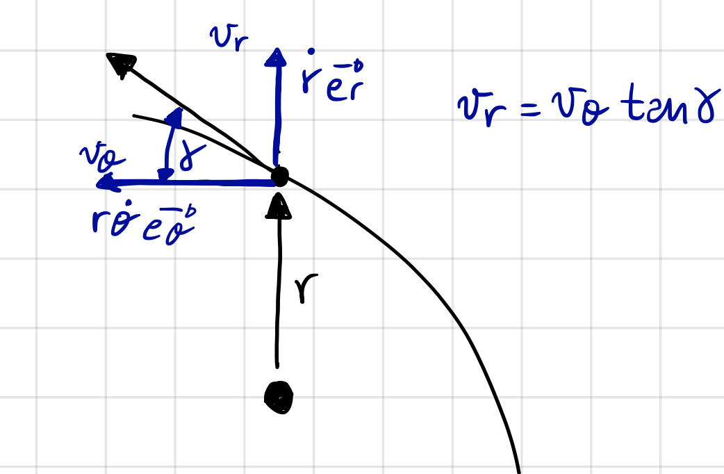
Fig. 12 Polar coordinate velocity components and the flight path angle.

In the above figure, the angle marked \(\gamma\) is the flight path angle; the angle between the tangential velocity vector \(\mathbf{v}_\theta\) and the velocity vector \(\mathbf{v}\). A trigonometric relationship between the flight path angle and the velocity components can be expressed using Fig. 12:

(138)\[\tan \gamma = \frac{v_r}{v_\theta}\]

By substituting Equations (136) and (137) for \(v_r\) and \(v_\theta\) respectively and simplifying, we obtain:

(139)\[\tan \gamma = \frac{e \sin \theta}{1 + \cos \theta}\]

Note

Additionally, we can make the following observations:

1. Tangential Component, \(v_\theta\)

   • \(v_\theta \geq 0\)

   • \(v_\theta\) is at its maximum when \(\theta = 0^\circ\) (perigee)

   • \(v_\theta\) is at its minimum when \(\theta = 180^\circ\) (apogee)

2. Radial Component, \(v_r\)

   • \(v_r \geq 0\) when \(0^\circ \leq \theta \leq 180^\circ\)

   • \(v_r < 0\) when \(180^\circ < \theta < 360^\circ\)

   • \(v_r = 0\) at \(\theta = 0^\circ\) (perigee) and \(\theta = 180^\circ\) (apogee). At these points, the motion is purely tangential.

The Perifocal Frame

The unit vectors (\(\mathbf{\hat{e}}_r\), \(\mathbf{\hat{e}}_\theta\)) in the polar coordinate system change along the orbital path, varying from point to point. A non-accelerating (i.e., inertial) reference frame can be established using three mutually perpendicular vectors that remain fixed relative to the orbital path. We have actually already identified two of these over the course of the previous discussions; they are

Recall:

• The specific angular momentum vector (\(\mathbf{h}\)) is a constant and is orthogonal to the plane of motion (i.e., the orbital plane).

• The eccentricity vector (\(\mathbf{e}\)) lies in the plane of motion and is directed towards the perigee.

A third vector, \(\mathbf{\hat{q}}\), can be defined as the cross product of \(\mathbf{h}\) and \(\mathbf{e}\) which together with \(\mathbf{e}\) and \(\mathbf{h}\) forms a set of three mutually perpendicular vectors. This set of vectors constitutes a frame fixed in the orbit known as the ** perifocal frame** and is illustrated in Fig. 13.

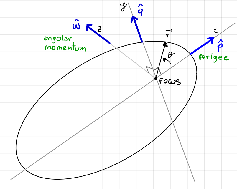
Fig. 13 Illustration of an elliptical orbit with the perifocal reference frame.

Creating the Perifocal Frame:

The following three unit vectors form an inertial reference frame, centered at the focus of the orbit:

1. The first vector, \(\mathbf{\hat{p}}\), is the unit vector in the direction of the eccentricity vector (\(\mathbf{e}\)).

(140)\[\mathbf{\hat{p}} = \frac{\mathbf{e}}{|\mathbf{e}|} = \frac{\mathbf{e}}{e}\]

2. The second vector, \(\mathbf{\hat{w}}\), is the unit vector in the direction of the specific angular momentum vector (\(\mathbf{h}\)), perpendicular to the plane of motion.

(141)\[\mathbf{\hat{w}} = \frac{\mathbf{h}}{\left|\mathbf{h}\right|} = \frac{\mathbf{h}}{h}\]

3. The third vector, \(\mathbf{\hat{q}}\), is obtained by taking the cross product of \(\mathbf{\hat{w}}\) and \(\mathbf{\hat{p}}\). Recall that the cross product of two vectors yields a vector that is perpendicular to both, ensuring that (\(\mathbf{\hat{p}}\),\(\mathbf{\hat{q}}\),\(\mathbf{\hat{w}}\)) is a set of three mutually perpendicular vectors.

(142)\[\mathbf{\hat{q}} = \mathbf{\hat{w}} \times \mathbf{\hat{p}}\]

Position Vector in the Perifocal Frame

From Fig. 13,

(143)\[\mathbf{r} = r \cos\theta \mathbf{\hat{p}} + r \sin\theta \mathbf{\hat{q}}\]

Position Vector in the Perifocal Frame

By substituting Equation (81) for \(r\) into the above equation, we obtain:

(144)\[\mathbf{r} = \frac{h^2 / \mu}{1 + e \cos\theta} \left( \cos\theta \mathbf{\hat{p}} + \sin\theta \mathbf{\hat{q}} \right)\]

Velocity Vector in the Perifocal Frame

The velocity vector can be obtained by differentiating the position vector (expressed in the perifocal frame, Equation (144)), with respect to time.

(145)\[\mathbf{v} = \frac{\mathrm{d} \mathbf{r}}{\mathrm{d} t} = \frac{\mathrm{d}}{\mathrm{d} t} \left( r \cos\theta \mathbf{\hat{p}} \right) + \frac{\mathrm{d}}{\mathrm{d} t} \left( r \sin\theta \mathbf{\hat{q}} \right)\]

Applying the product rule to each term:

\[\frac{\mathrm{d}}{\mathrm{d} t} \left( r \cos\theta \mathbf{\hat{p}} \right) = \dot{r} \cos\theta \mathbf{\hat{p}} + r \left( -\sin\theta \dot{\theta} \right) \mathbf{\hat{p}}\]

\[\frac{\mathrm{d}}{\mathrm{d} t} \left( r \sin\theta \mathbf{\hat{q}} \right) = \dot{r} \sin\theta \mathbf{\hat{q}} + r \left( \cos\theta \dot{\theta} \right) \mathbf{\hat{q}}\]

Combining these results:

\[\frac{\mathrm{d} \mathbf{r}}{\mathrm{d} t} = \left( \dot{r} \cos\theta - r \dot{\theta} \sin\theta \right) \mathbf{\hat{p}} + \left( \dot{r} \sin\theta + r \dot{\theta} \cos\theta \right) \mathbf{\hat{q}}\]

Recalling that, \(v_r = \dot{r}\) and \(v_\theta = r \dot{\theta}\), from Equation (128), the expression for the velocity vector becomes:

\[\frac{\mathrm{d} \mathbf{r}}{\mathrm{d} t} = \left( v_r \cos\theta - v_\theta \sin\theta \right) \mathbf{\hat{p}} + \left( v_r \sin\theta + v_\theta \cos\theta \right) \mathbf{\hat{q}}\]

By subsituting Equations (136) and (137) for \(v_r\) and \(v_\theta\) respectively, and simplifying, we arrive at:

Note again that the velocity vector is the perifocal frame is also two-dimensional.

Velocity Vector in the Perifocal Frame

(146)\[\mathbf{v} = \frac{\mathrm{d} \mathbf{r}}{\mathrm{d} t} = \frac{\mu}{h} \left( -\sin\theta \mathbf{\hat{p}} + \left(e + \cos\theta \right) \mathbf{\hat{q}} \right)\]

With Equations (144) and (146), we can express the position and velocity of the spacecraft in the perifocal frame, which is an inertial frame of reference.

The ECI Reference Frame

Up to this point, we’ve described the orbit in its orbital plane, which is a 2D description. Although the perifocal frame is 3D, it is orbit-dependent. We seek a more general description. To define an inertial frame, we need:

1. An origin

2. The direction of two fixed normal vectors (the third is automatically determined by the cross product of the two known vectors). Based on this, we define the Earth Centred Interial (ECI) Frame.

Earth Centred Interial (ECI) Frame

ECI frame is an inertial frame of reference with:

• Origin at the Earth’s centre of mass

• \(z\)-axis aligned with the Earth’s spin axis

• \(x\)-axis aligned with the first the First Point of Aries, \(\gamma\)

Key Terms:

• Ecliptic Plane: the plane of the Earth’s orbit around the Sun

• Equatorial Plane: the imaginary plane extending outwards from the Earth’s celestial equator

• Vernal Equinox: the intersection line of the Earth’s equatorial plane and the ecliptic plane, indicating the direction of the First Point of Aries

• Obliquity (\(\epsilon\)): the angle between the Earth’s spin axis (normal to the equatorial plane) and the normal to the ecliptic plane

These are illustrated in Fig. 14.

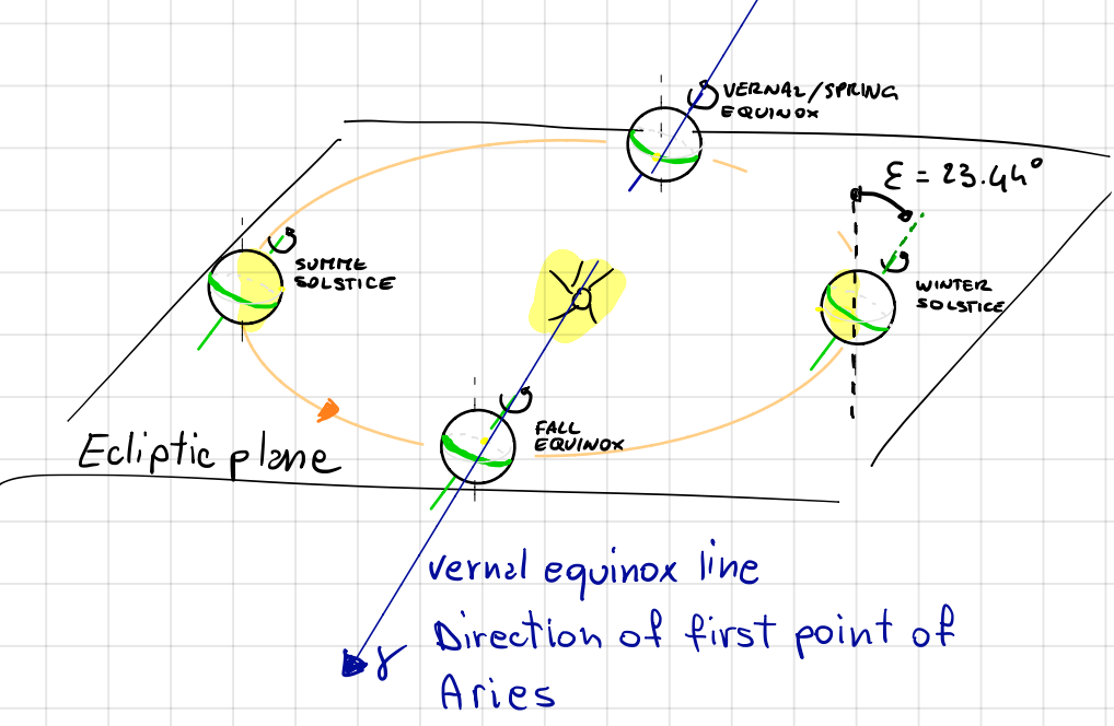
Fig. 14 Diagram of the Earth’s orbit around the Sun, showing the ecliptic and equatorial planes (the plane formed when the green line is extended radially outwards), the direction of the First Point of Aries, and the obliquity angle.

• As seen from Earth, the sun moves on the ecliptic counterclockwise as shown in Fig. 15.

• The direction of the First Point of Aries is defined when the Sun crosses the equatorial plane from south to north.

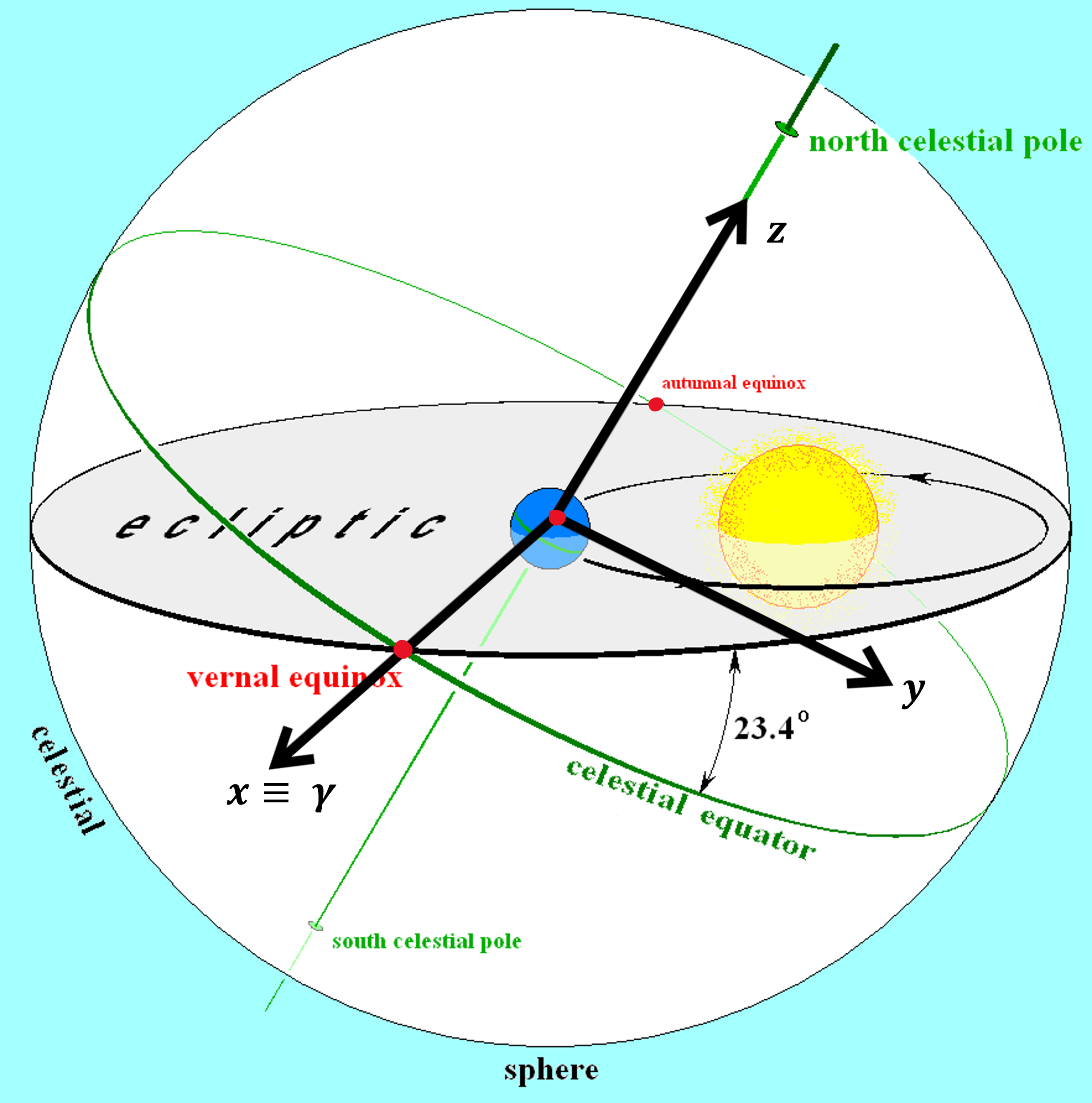
Fig. 15 Diagram of Earth’s orbit, illustrating ecliptic plane and celestial equator on the celestial sphere. The three orthogonal vectors that define the ECI frame have also been labelled.

Problem:

The coordinate system \(x-y-z\) show in Fig. 15 is not inertial, due to:

• Precession (and nutation) of the spin axis: Caused by the gravitational pull of the Sun and Moon combined with the Earth’s oblateness.

• Precession of the ecliptic plane: Due to the gravitational pull exerted by other planets on the Earth.

• \(\gamma\) completes a full revolution in approximately 26,000 years, with a superimposed nutation of about 0.005° with a period of 18.6 years.

Solution:

To address this, we work with \(x-y-z\) axes at a given epoch, for example, the ECI J2000 (or J2K) reference frame.

The Celestial Sphere

The celestial sphere is an imaginary, infinitely large sphere (shown in Fig. 15 and Fig. 16) centered on the Earth, onto which all celestial objects are projected. The positions of these objects are defined by:

1. Right Ascension (\(\alpha\)): measured in the positive (+) direction eastward along the celestial equator from the vernal equinox.

2. Declination (\(\delta\)): measured in the positive (+) direction northward from the celestial equator.

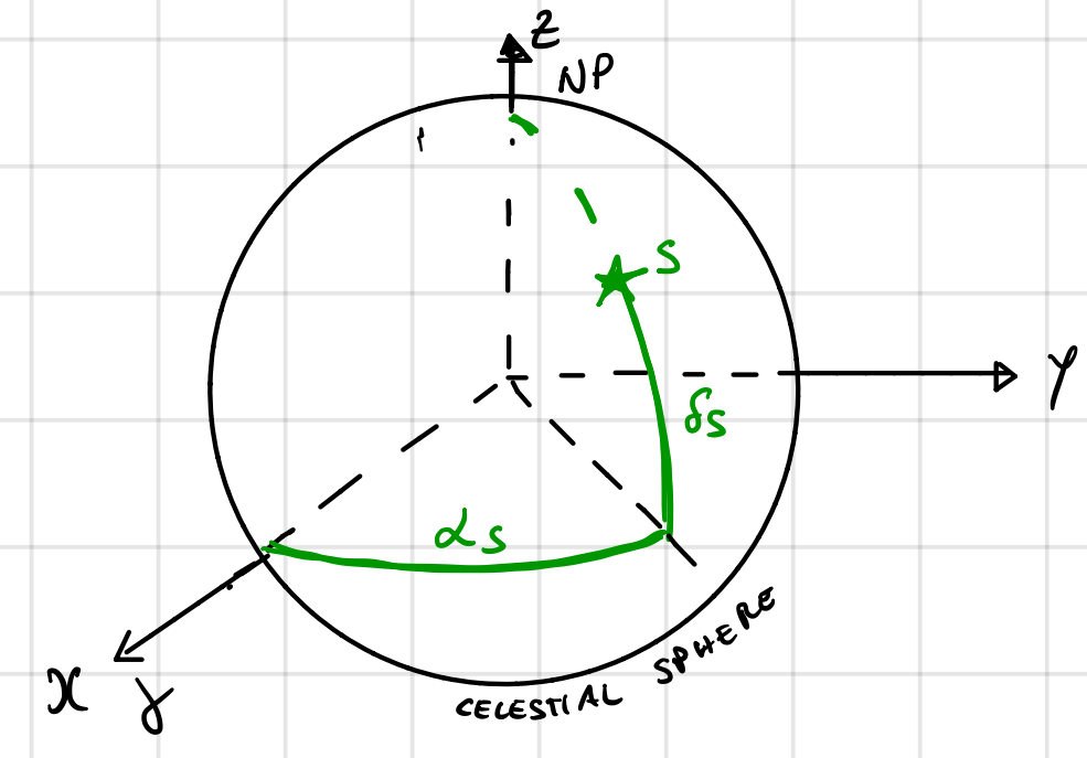
Fig. 16 Diagram of the celestial sphere showing the right ascension and declination.

Classical Orbital Parameters

A general orbit can often be described using what are known as the six “classical orbital elements”.

• The orbit’s shape is defined entirely by the semi-major axis (\(a\)) and eccentricity (\(e\)), which are both constants.

• The position along the orbit is given by the true anomaly, \(\theta(t)\). This is solved for with Kepler’s Equation.

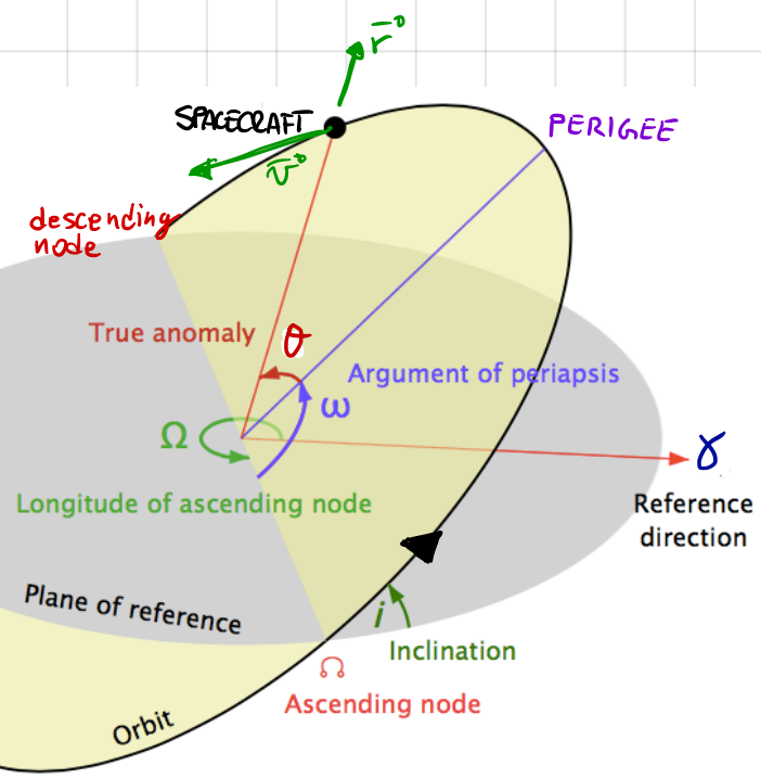
Fig. 17 Diagram illustrating the classical orbital parameters.

For a complete 3D representation, two additional parameters define the orbital plane, and another parameter specifies the orientation of the line of apsides within that plane. All of these orbital parameters can be seen in Fig. 17 and are discussed in further detail below.

1. The Orientiation of the Plane

• Right Ascension of Ascending Node (\(\Omega\), also referred to as the Longitude of Ascending Node), represents the angle from the \(x\)-axis to the intersection point (the ascending node) of the equatorial and orbital planes. It varies between \(0^\circ\) and \(360^\circ\) (i.e., \(\epsilon[0,360]\)).

• Inclination (\(i\)), is the angle between the equatorial and orbital planes. Though \(\epsilon[0,180]\),

  • the orbit is prograde when \(0^\circ < i < 90^\circ\)

  • the orbit is retrograde when \(90^\circ < i < 180^\circ\)

2. The Direction of Perigee

• Argument of perigee (\(\omega\)), is the angle between the ascending node and the perigee. Remember when \(e=0\), there is not a single point in the orbit closest to the central body as it’s a circular orbit. \(\epsilon[0,360]\)

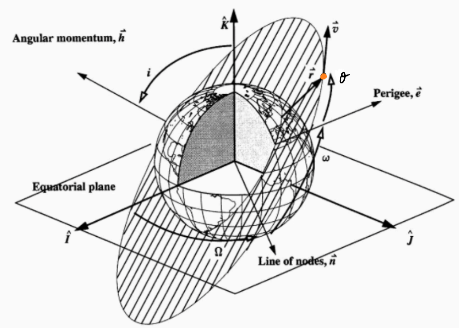
Fig. 18 Diagram illustrating the key parameters and angles used in the context of a satellite orbiting the Earth.

Fig. 18 shows some of these parameters for an Earth-orbiting satellite.

• \(\Omega\) is the angle between \(\mathbf{\hat{I}}\) and the line of nodes \(\mathbf{\hat{n}}\). Recall that the line of nodes connects the ascending and descending nodes, which are the points where the orbital plane intersects the equatorial reference frame. Therefore, the line of nodes lies in both planes and is perpendicular to the normal vectors of both the reference plane and the orbital plane. In other words:

\[\mathbf{\hat{n}} = \mathbf{\hat{K}} \times \mathbf{h}\]

where

• \(i\) is the angle between \(\mathbf{h}\) and \(\mathbf{\hat{K}}\)

• \(\omega\) is the angle between \(\mathbf{e}\) and \(\mathbf{n}\)

Note:

• Given \(h, e = const\), we are able to say \(a\), \(e\), \(i\), \(\omega\) and \(\Omega\) are all constants.

• The only orbital parameter that varies with time is \(\theta\), which is determined by solving Kepler’s equation.