Circular and More Results on Elliptical Orbits

Prepared by: Ilanthiraiyan Sivagnanamoorthy, Joost Hubbard, and Angadh Nanjangud

In this lecture we aim to cover the following topics:

1. Properties of Circular Orbtis

2. Orbital Period (Kepler’s 3rd Law)

3. r as a function of time

Properties of Circular Orbtis

1. Orbital Radius (\(r\))

Recall that the equation of the orbit in Equation (81) was based on the semi-latus rectum (\(p\)) and can be written as:

(90)\[r = \frac{p}{1 + e \cos (\theta)}\]

For a circular orbit, the eccentricity (\(e\)) is 0. Substituting \(e = 0\) into Equation (90) simplifies it to:

(91)\[r = p\]

In this case, the semi-latus rectum (\(p\)) is equal to the semi-major axis (\(a\)), since:

(92)\[p = a(1-e^2) = a\]

Thus, for a circular orbit,

Important

(93)\[r = p = a= const\]

2. Orbital Velocity (\(v\))

Equation (89) gives the vis-viva equation, which we rewrite to solve for the orbital velocity (\(v\)) of an object given its distance from the planet’s center (i.e., orbital radius, \(r\)) and the semi-major axis (\(a\)) of this orbit.

(94)\[v^2 = \mu \left( \frac{2}{r} - \frac{1}{a} \right)\]

For a circular orbit, the relationship between \(r\) and \(a\) has been defined in Equation (93). Substituting this into Equation (94) yields the following equation for the orbital velocity:

Important

(95)\[v = \sqrt{\frac{\mu}{a}}\]

3. Radial (\(v_r\)), transverse (\(v_\theta\)), and angular speeds (\(\dot{\theta}\))

Recall that the velocity vector in polar coordinates can be expressed as:

(96)\[\begin{split}{\bf v} &= v_r\mathbf{\hat{e}}_r + v_\theta\mathbf{\hat{e}}_\theta\\ &= \dot r\mathbf{\hat{e}}_r + r \dot \theta\mathbf{\hat{e}}_\theta\end{split}\]

from Equations (47) and (53).

Since orbital radius \(r\) is a constant for a circular orbit, also provided in Equation (93), the radial component of \({\bf v}\) is 0. Thus, we get that

(97)\[v_r = \dot r = \frac{dr}{dt} = 0\]

and the velocity vector of Equation (96) simplifies to include only the transverse component:

(99)\[\begin{split}{\bf v} &= v_r \\ &= r \dot \theta\mathbf{\hat{e}}_\theta\end{split}\]

This tells us that the transverse velocity component \(v_\theta\) is given by comparing Equations (99) and (95):

Important

(99)\[v_\theta = v = \sqrt{\frac{\mu}{a}}\]

By equating the magnitude of \({\bf v}\) given by Equation (99) to that given by Equation (95), we can solve for angular speed \(\dot{\theta}\) as follows:

(101)\[v = r \dot \theta = a \dot \theta = \sqrt{\frac{\mu}{a}}\]

or

Important

(101)\[\dot \theta = \sqrt{\frac{\mu}{a^3}}\]

As \(a = const\) for circular orbits and \(\mu = const\) in the two-body problem, Equation (101) proves that the angular speed (and therefore the angular velocity) is also a constant.

So, the angular position of a body in a circular orbit is given by:

(103)\[\theta = \sqrt{\frac{\mu}{a^3}}(t-t_0)\]

where \(t_0\) is the time passage from a reference direction.

4. Orbital Period (\(T\))

Equation (101) is used to define the orbital time period as:

(103)\[T = \frac{2\pi}{\dot \theta} = 2\pi\sqrt{\frac{a^3}{\mu}}\]

The concept of orbital period is discussed in detail in the next section.

Orbital Period (Kepler’s 3rd Law)

Kepler’s 2nd law of planetary motion states that an object in orbit sweeps out equal areas in equal time intervals, meaning the areal velocity is constant. This law is expressed in terms of specific angular momentum (\(h\)) as:

(104)\[\frac{dA}{dt} = \frac{1}{2}h = const\]

Given that \(h = \sqrt{\mu p}\) and \(p = a(1-e^2)\), Equation (104) can be rewritten as:

(105)\[\frac{dA}{dt} = \frac{1}{2}\sqrt{\mu a (1-e^2)}\]

The orbital period (\(T\)) is the time the spacecraft takes to complete a full revolution. During this period, the spacecraft sweeps out the entire area of the ellipse, which is given by:

(106)\[A_T = \pi ab = \pi a^2 \sqrt{1-e^2}\]

Using Equation (106), the areal velocity can be expressed as:

(107)\[\frac{dA}{dt} = \frac{A_T}{T} = \frac{\pi a^2 \sqrt{1-e^2}}{T}\]

Equating Equations (105) and (107) to derive an equation for the orbital period and then rearranging gives:

Important

(108)\[T = 2\pi \sqrt{\frac{a^3}{\mu}}\]

The equation above defines Kepler’s 3rd law, which states that the square of the orbital period is proportional to the cube of the semi-major axis (i.e., \(T^2 \propto a^3\)).

• \(T\) can be used to measure \(m_2\) (the mass of the central body)

• \(T\) (and energy) are independent of the eccentricity of the orbit

By defining a parameter called the mean motion (\(n\)) as \(2\pi/T\), Equation (108) can be alternatively expressed as:

Important

(109)\[n^2 a^3 = \mu\]

\(r\) as a function of time

The Objective

Equation (90) represents Kepler’s 1st law, which states that the orbit of a planet is an ellipse with the sun at one of its two foci. This equation provides \(r\) as a function of \(\theta\), i.e., \(r(\theta)\), but it does not explicitly give \(r\) as a function of time, i.e., \(r(t)\). In the following passage, our goal is to determine \(\theta(t)\), so that we can find \(r(\theta(t))\), which then gives us \(r(t)\).

Derivation

Starting with the magnitude of the specific angular momentum, \(h = r^2 \dot\theta\), and substituting Equation (90) for \(r\), then rearranging to solve for \(\dot \theta\) results in Equation (110). Note that Equation (90) was originally expressed in terms of the semi-latus rectum (\(p\)), but in the following steps, \(p\) has been replaced with \(\frac{h^2}{\mu}\) as per Equation (82).

(110)\[\dot{\theta} = \frac{d\theta}{dt} = \frac{h}{r^2} = \frac{\mu^2}{h^3}\left(1 + e \cos(\theta)\right)^2\]

We rearrange the above equation to integrate the equations by separation of variables, with \(\theta\) on the LHS and \(t\) on the RHS:

(111)\[\int \frac{d\theta}{\left(1 + e \cos(\theta)\right)^2} = \int \frac{\mu^2}{h^3} \, dt\]

The integration results in:

Important

(112)\[\frac{\mu^2}{h^3} (t - t_p) = \int_{0}^{\theta} \frac{d\theta}{\left(1 + e \cos(\theta)\right)^2}\]

• \(t_p\) is the time of perigee passage, which is the specific moment when the orbiting object is closest to the primary body it is orbiting. For simplicity, we assume \(t_p = 0\).

• The true anomaly (\(\theta\)) is measured from the eccentricity vector (\(\bf{e}\)), which is aligned with the line of apsides and directed towards the perigee point. By assuming \(t_p = 0\) we have \(\theta(t_p) = \theta(0) = 0\).

• Solving Equation (112) results in \(\theta(t)\). We defined this as our objective!

Case 1. Circular Orbits

Given \(e = 0\) for circular orbits and the assumed \(t_p= 0\), Equation (112) is reduced to:

(113)\[\frac{\mu^2}{h^3}t = \theta\]

Since \(p = h^2/\mu\) and that \(p = a = const\) for circular orbits, the above may be expressed in terms of \(a\) as follows:

(114)\[\begin{split}\theta &= \frac{\mu^2}{(\mu a)^\frac{3}{2}}t\\ &= \frac{\mu^\frac{1}{2}}{(a)^\frac{3}{2}}t\\ &= \sqrt{\frac{\mu}{a^3}}t\end{split}\]

This relation can be further simplified using Kepler’s third law, Equation (108) and compactly expressed in terms of the mean motion \(n\),

(115)\[\begin{split}\theta &= \frac{2\pi}{T}t\\ \Rightarrow \theta &= nt\end{split}\]

Case 2. Elliptical Orbits

Given \(0<e<1\) for elliptical orbits and assuming \(t_p = 0\), Equation (112) evaluates to:

\[\frac{\mu^2}{h^3}t = \frac{1}{(1 - e^2)^{3/2}} \left[ 2 \tan^{-1} \left( \sqrt{\frac{1 - e}{1 + e}} \tan \left(\frac{\theta}{2}\right) \right) - \frac{e \sqrt{1 - e^2} \sin(\theta)}{1 + e \cos(\theta)} \right]\]

By multiplying out the denominator term on the right-hand side of the equation, we obtain:

(116)\[\frac{\mu^2}{h^3} (1 - e^2)^{3/2} t = 2 \tan^{-1} \left( \sqrt{\frac{1 - e}{1 + e}} \tan \left(\frac{\theta}{2}\right) \right) - \frac{e \sqrt{1 - e^2} \sin(\theta)}{1 + e \cos(\theta)}\]

Mean Anomaly (for general elliptical orbits)

The term on the LHS of Equation (116) is a parameter for elliptical orbits often referred to as the mean anomaly (\(M_e\)):

(117)\[M_e = \frac{\mu^2}{h^3}(1 - e^2)^\frac{3}{2}t\]

Thus, we rewrite Equation (116) as:

Important

(118)\[M_e = 2 \tan^{-1} \left( \sqrt{\frac{1 - e}{1 + e}} \tan \left(\frac{\theta}{2}\right) \right) - \frac{e \sqrt{1 - e^2} \sin(\theta)}{1 + e \cos(\theta)}\]

We can also derive a simpler expression for the mean anomaly of an elliptical orbit from the orbital period given by Equation (108), \(T = 2\pi \sqrt{\frac{a^3}{\mu}}\). Here, we invoke the definition of the semi-latus rectum from Equation (82), \(p = a(1-e^2) = h^2/\mu\), to get an expression for \(a\) in terms of \(h\) and \(\mu\)

\[a = \frac{h^2}{\mu(1-e^2)}\]

and subsequently substitute for \(a\) in this expression for \(T\) to get:

\[\begin{split}T &= 2\pi \sqrt{\frac{h^6}{\mu^3(1-e^2)^3}\frac{1}{\mu}}\\ \Rightarrow T &= 2\pi \frac{h^3}{\mu^2(1-e^2)^\frac{3}{2}}\end{split}\]

Rearranging the above to express it as:

(119)\[\frac{2\pi}{T} = \frac{\mu^2}{h^3}(1-e^2)^\frac{3}{2}\]

Substituting Equation (119) and subsequently the definition of mean motion (\(n\)) into Equation (117), it can be reduced to:

Important

(120)\[M_e = \frac{2\pi}{T}t = nt\]

• From this definition, the mean anomaly can be interpreted as the angular position of a fictitious body moving around the ellipse at constant angular speed \(n\).

• This hypothetical body travels around the orbit in such a way (with constant angular speed) that it completes one full revolution in the same period \(T\) as the actual body.

• The real body in an elliptical orbit, however, would speed up and slow down due to gravitational forces, whilst holding the areal velocity constant (i.e., Kepler’s 2nd Law).

• If the ellipse has zero eccentricity, then \(M_e = \theta\), as given by Equation (115).

Kepler’s Equation

Our objective here is to derive the most important equation of orbital mechanics, Kepler’s equation, by simplifying Equation (116).

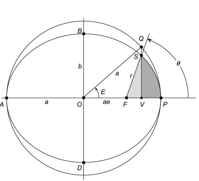
Fig. 10 An ellipse with a circumscribed reference circle, where the semi-major axis of the ellipse is equal to the radius of the circle.

In Fig. 10, the semi-major axis (\(a\)) of the orbital ellipse is equal to the radius of the circumscribed circle. An additional angle, called the eccentric anomaly (\(E\)), is introduced. Similar to the true anomaly (\(\theta\)), \(E\) is measured from the line of apsides and represents the angular position of the orbiting body as it would appear projected onto the reference circle. From this diagram, the following geometrical relationships can be derived:

(121)\[\overline{\bf OV} = a\cos(E)\]

but also

(122)\[\begin{split}\overline{\bf OV} &= \overline{\bf OF} + \overline{\bf FV}\\ \Rightarrow \overline{\bf OV} &= ae + r\cos(\theta)\end{split}\]

Then, equating the RHS of Equations (121) and (122), we get:

\[a\cos(E) = ae + r\cos(\theta)\]

Substituting for \(r\) (from Equation (90)) into the above equation and also then substituting for \(p = a(1-e^2)\):

\[\begin{split}a \cos(E) &= ae + \frac{p}{1 + e \cos(\theta)} \cos(\theta)\\ \Rightarrow a \cos(E) &= ae + \frac{a (1 - e^2)}{1 + e \cos(\theta)} \cos(\theta)\end{split}\]

which simplifies to:

(123)\[\begin{split}\Rightarrow \cos(E) &= e + \frac{(1-e^2)}{1+e\cos(\theta)}\cos(\theta)\\ \Rightarrow \cos(E) &= \frac{e + \cos(\theta)}{1 + e\cos(\theta)}\end{split}\]

The below Fig. 11 shows an ambiguity; a given value of \(\cos E\) (i.e., for a given value of \(\theta\)) corresponds to two possible values of \(E\):

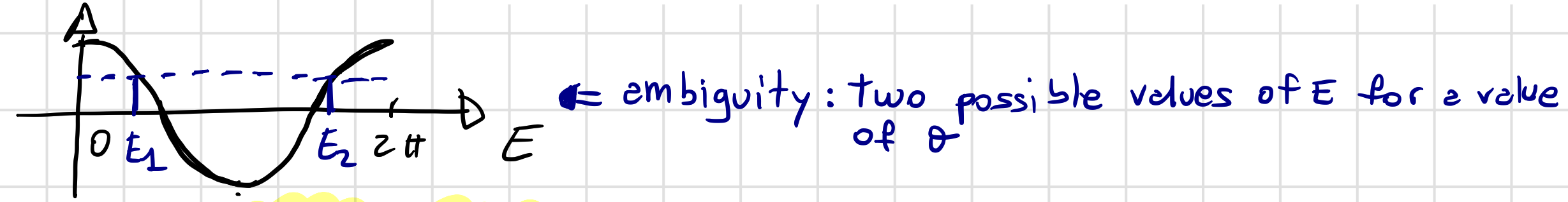
Fig. 11 Plot of \(\cos(E)\) against \(E\) from 0 to \(2\pi\) shows that there are two possible values of \(E\) for a given value of \(\cos(E)\).

This will need to be resolved to determine the correct value of \(E\) for a given value of \(\theta\).

We first use the trigonometric identity \(\sin^2(E) + \cos^2(E) = 1\) to derive an equation for \(\sin(E)\):

Important

(124)\[\sin(E) = \frac{\sqrt{1-e^2}\sin(\theta)}{1 + e\cos(\theta)}\]

Then, we introduce \(\tan^2(\frac{E}{2})\) and recall the half-angle formula for it in terms of \(\cos(E)\) as:

\[\tan^2(\frac{E}{2}) = \frac{1-\cos(E)}{1+\cos(E)}\]

Evaluate the above by substituting Equation (123) for \(\cos(E)\). This results in:

\[\tan^2(\frac{E}{2}) = \frac{1-e}{1+e}\tan^2(\frac{\theta}{2})\]

or

Important

(125)\[\tan(\frac{E}{2}) = \sqrt{\frac{1-e}{1+e}}\tan(\frac{\theta}{2})\]

If we compare the terms on the RHS of Equation (118) with the terms on the RHS of Equations (124) and (125), we can write:

\[M_e = 2 \tan^{-1} \left( \tan \left( \frac{E}{2} \right) \right) - e \sin(E)\]

or written in the form commonly known as Kepler’s equation:

Kepler’s equation

(126)\[M_e = E - e\sin(E)\]

As \(M_e\) can be represented in terms of the mean motion (\(n\)) as either \(nt\) or more generally as \(n(t - t_p)\), Kepler’s equation can alternatively be expressed as follows:

(127)\[n(t-t_p) = E - e\sin(E)\]

Kepler’s equation

Kepler’s equation is useful in two scenarios:

• Scenario 1: To determine the time since perigee passage given \(\theta\):

  1. Calculate the eccentric anomaly \(E\) using Equation (125).

  2. Compute the mean anomaly \(M_e\) from Kepler’s equation.

  3. Determine the mean motion \(n\) using \(n = 2\pi/T\) or Equation (109).

  4. Find the time since perigee passage with \(t-t_p = M_e/n\).

Important

• Scenario 2: To determine \(\theta\) when given \(t\):

  1. Compute the mean motion \(n\) using \(n = 2\pi/T\) or Equation (109).

  2. Calculate the mean anomaly \(M_e = n(t-t_p)\).

  3. Solve Kepler’s equation numerically to find the eccentric anomaly \(E\).

  4. Compute \(\theta\) from Equation (125)